- Details
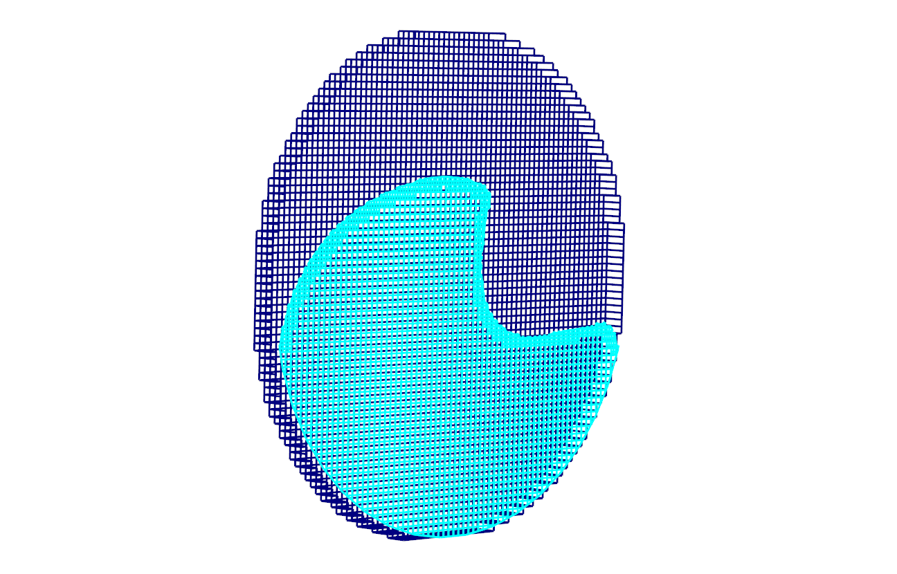
In this article we will be discussing the computational grid. FlowVision uses a structured locally adaptive mesh with sub-grid resolution of geometry, predominantly consisting of hexagonal cells. The computational grid is constructed automatically. The accuracy of the mesh refinement of a geometric model of any complexity is ensured by using a technology for sub-grid geometry resolution.
If you would like to know more, read on for our answers to the 5 most frequent questions about the FlowVision grid:
1. How to construct a computational grid in FlowVision?
2. What is "adaptation" of the computational grid?
3. How to evaluate mesh quality in FlowVision?
4. I have a complex geometric model. How can the FlowVision mesh ensure accuracy of the calculation in boundary cells?
5. The computational grid and moving bodies: how do they interact during the computation process?
- Details
Characteristics are one of the most powerful tools in the FlowVision software complex for obtaining information about the calculation.
Characteristics can be used to:
- obtain calculation results, such as: flow rate, pressure, temperature, or forces acting on a surface or in a volume section
- monitor calculation results, outputting the data as a graph within the program interface
- debug the project / diagnose problems (for example, by finding extreme values within the computational space).
- Details
Advanced users of FlowVision are certainly familiar with the trick of using a remote non-computational subdomain for 2D simulations that utilise grid adaptation. This non-obvious method is used to disable mesh adaptation along one coordinate direction, thus making sure there will be only one cell across the width of the computational space. Despite being complicated, the trick works and helps to minimize computational mesh in 2D simulation.
In the new release of FlowVision, the 2D-simulation option is built into the program interface. Now you can create a project with 2D adaptation in just one click. Furthermore, the creation of projects with a 2D-sector condition has become easier.
You can try it! In this article we'll be talking about why it's so important to first perform a 2D calculation instead of directly jumping into a 3D one.

- Details
For the first time in our blog - the whole article is devoted to the FVTerminal module! If you want to speed up and automate the start of your simulations, then you just need to get acquainted with its capabilities.
FVTerminal allows you to perform certain operations while bypassing FVPPP, and can also do other cool things:
- start and stop calculation (on local and remote computers)
- download the client part of the project form the server part data
- delete projects permanently
- connect to the Solver via the Viewer
- and most interesting of all - queue projects

- Details
Today's topic is not how to obtain and install FlowVision license - this information can be found in our earlier blog articles or requested from our sales manager. Let's talk instead about when you would need a FlowVision license and when you can work without one. And also a little about licensing options and the error "No free licenses for this user".
- Details
Welcome to the FlowVision users team! Before you start creating your first project, you need to download the distribution pack and prepare it for work. In this article, we will tell you how to do this, so you can begin simulation of your engineering tasks as quickly as possible.
Here are the steps that will help get you absolutely prepared to run local FlowVision simulations on PC:
Step 1: Download FlowVision and License Manager
Step 2: Install FlowVision and License Manager
Step 3: Register the license
Step 4: Create Solver-Agent user
Step 5: Check the license settings
- Details
This functionality provides many opportunities for increasing accuracy of calculations while using less computational resources.
For your tasks, you can use:
- volume / surface adaptation;
- adaptation for curvature / sharp edges;
- adaptation by condition / to solution;
- merging.
- Details
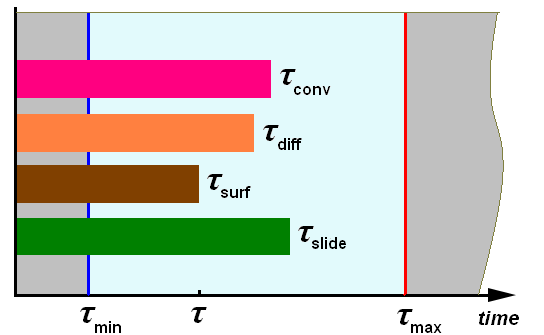
To solve a numerical task, it is necessary to discretize space and time. A time scale allows to find intermediate solutions based on the initial and boundary conditions. Gradually coming through the intermediate solutions, we get the final one, which we can use to achieve the goals: choosing the right paint for the rocket skin, calculating the flow rate of your favorite ketchup, or getting the optimal washing temperature for a cat.
The intervals at which software calculates a solution are commonly referred to as the time step. It can be constant or calculated for each iteration based on a certain criteria. It should be noted that the time step is different for each specific software and task.
How to specify it correctly - we will describe in this article.
- Details
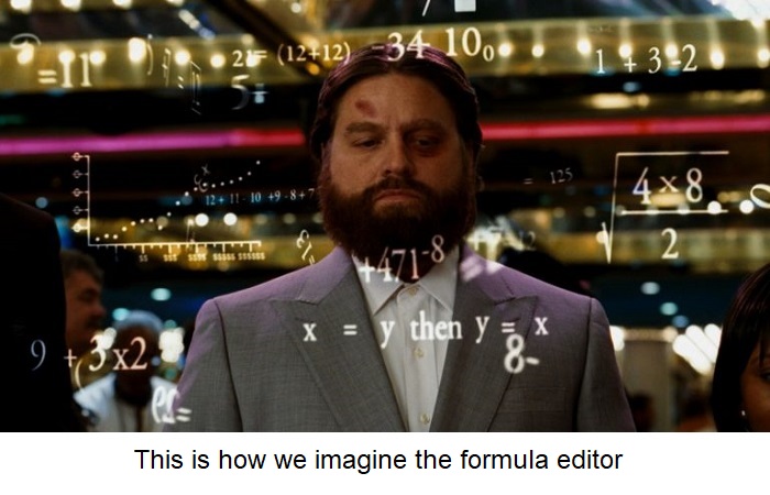
You can use formulas in FlowVision to set any variable: from the gravity vector to the law of a moving body motion. All this became possible with the formula Editor. Using the formula Editor you may calculate composite functions, set the physical laws of variable changings and even set the level of adaptation for the calculation grid depending on the step number (and much more!).
In this article we will show how this functionality can significantly simplify the user's life.
- Details
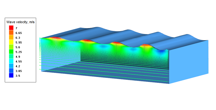
Now it's easier to simulate sea waves in FlowVision!
You may set complex boundary conditions for the formation of natural gravitational waves using the formula editor. But these formulas are quite complex. Therefore, we used the computational engineering platform API and connected this module to FlowVision, so it became convinient to create user boundary conditions which generate waves.
- Details
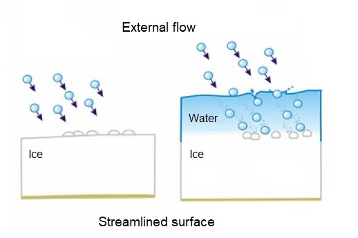
For FlowVision 3.12.01 release we made a breakthrough in the development of processes in dispersed phases. As a result, it became possible to simulate the icing of surface. Today you can apply the both icing modes to your tasks - dry icing mode and wet one. What is the difference between these modes? How to simulate icing processes correctly? What results will be obtained in FlowVision? You will find all answers in this article.
- Details
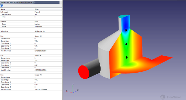
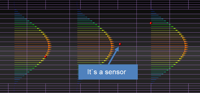
A set of sensors is a measuring object which can be placed anywhere in the calculation domain.
Previously, to obtain a variable at a certain point of computational domain, it was necessary to create a small object with dimentions closed to the cell size and set a characteristic on this object. It became much more convenient with the help of sensors. You can simply select a point or even several points in space, create there the sensor set and receive data in one glo-file.