WHAT IS "ADAPTATION" OF THE COMPUTATIONAL GRID?
Grid adaptation is the splitting of mesh cells into smaller ones used for local solution refinement.
Adaptation can be applied to those areas of the computational domain in which it is necessary to refine the solution: for example, in the near-wall layer or in regions with steep gradients, etc. In FlowVision, you can adapt the mesh:
- at the surface or within the volume of geometric objects (you can also further adapt sharp corners and curved surfaces – regions where the flow changes and large gradients appear)
- at the surface of boundary conditions
- in regions with large gradients of parameters or with a certain value of a specific parameter.
When standard 3D adaptation is enabled, the initial-level computational cells are split in half in all three directions, resulting in 8 smaller cells. Initial grid cells have adaptation level 0. With a single partition of the initial grid, cells with adaptation level 1 are formed. With further partitioning the adaptation level sequentially increases, accordingly.
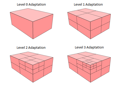
A level 0 cell is adapted to level 3
Adaptation is not only the splitting, but also the combining of cells into larger ones (but not larger than the initial level 0 cell size). In FlowVision, this is called merging.
The combination of periodic merging and mesh refinement using adaptation by condition means you can have dynamic mesh adaptation in FlowVision. It then becomes possible to refine the mesh only in the areas that require finer mesh resolution for solution accuracy, whereas excess adaptation in the rest of the computational space merges back to lower levels on account of being unnecessary.

Dynamic adaptation by density in supersonic flow around a wedge: using adaptation by condition + merging