In this article we will be discussing the computational grid. FlowVision uses a structured locally adaptive mesh with sub-grid resolution of geometry, predominantly consisting of hexagonal cells. The computational grid is constructed automatically. The accuracy of the mesh refinement of a geometric model of any complexity is ensured by using a technology for sub-grid geometry resolution.
If you would like to know more, read on for our answers to the 5 most frequent questions about the FlowVision grid:
FlowVision uses a structured locally adaptive mesh with sub-grid resolution of geometry, predominantly consisting of hexagonal cells
The main feature of the computational grid FlowVision is the speed with which it is generated. The user only needs to specify the number of grid lines in each Cartesian coordinate direction (to build a uniform grid) or specify the cell size and refinement reference lines in the initial-grid editor (to build a non-uniform grid). After that, the program will quickly automatically generate the mesh.
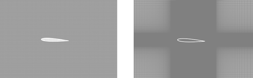
Uniform mesh (left) and non-uniform mesh with increased density near the profile (right)
Adaptations are used to refine the mesh cells in order to get a more accurate local solution. In FlowVision you can adapt the mesh on boundary conditions, as well as on the surface or within the volume of geometric objects. Conditional adaptation or adaptation to solution can be used to adapt the mesh based on local key parameter values within the simulation. Adaptation can be used not only to refine the mesh, but also to undo the splitting of cells (up to the initial level) - this is called merging. Merging of adaptations allows the use of dynamic adaptation methods that change throughout the simulation process. This approach allows you to, throughout the calculation, resolve (refine) only those regions containing parameter values of interest, while conserving computational resources (in areas where adaptation is no longer needed, it will be removed by merging the cells).
A more precise resolution of the viscous boundary layer is made possible by the subsurface mesh. This technology helps achieve detailed mesh refinement in the near-wall region along with significant computational savings when compared to regular 3D adaptation.
It may seem that refinement of the computational grid is a necessary condition for obtaining an accurate, precise solution in CFD solvers. But in FlowVision this is not always the case. For example, by using the gap model, it becomes possible to obtain an accurate solution in narrow channels and gaps without the need for mesh refinement.
HOW TO CONSTRUCT A COMPUTATIONAL GRID IN FLOWVISON?
Generating the initial grid in FlowVision is easy. The grid is constructed automatically in accordance with the specified parameters which can be either the number of lines of uniform division in each Cartesian direction, or the cell size and the position of refinement lines for higher grid density.
You can see the ease of meshing in FlowVision for yourself in this video about working with the Initial Mesh Editor.