- Details
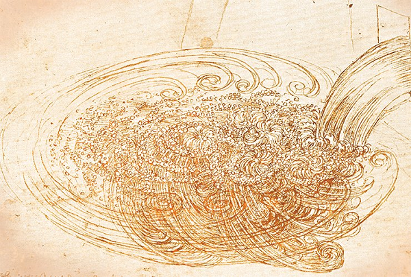
This article will be useful for the beginners who want to learn more about the turbulent flow and pitfalls encountered during its modeling. We'll go through:
- Details
FlowVision 3.11.01 obtained a new connector for linking to Abaqus. The new connector calls Abaqus CSE. This connector expands possibilities of direct coupling connector and has following advantages:
- More flex settings of co-simulation;
- Easier launching at cluster machines;
- Introducing of additional programs into co-simulation;
- Interaction with newest version of SIMULIA Abaqus.
Such advantages are realizing by Abaqus module: Abaqus CSE Director. But such approach has his own disadvantages:
- Abaqus CSE Director requires configuration file for his work;
- Complex launching of Abaqus which is not supporting by MPM-Agent of current FV version.
The problem of file generation was resolved. FlowVision creating file by user request. As input data FlowVision use Abaqus project which needed for connector creating.
Analysis launching by MPM-Agent has problems with commands which are transferring to Abaqus: are separated launching of Abaqus CSE Director and separated launching of project.
Script was created for resolving this problem and making launching of Abaqus more simple. This script taking data from FlowVision project and allows launching both type of connectors: Direct coupling and Co-simulation Engine.
Script as for Windows OS, as for Linux OS is attached to this paper for using.
- Details
There are many improvements in new version of FlowVision 31001. They significantly concern to functionality of adjusting and editing of computational grid such as computational grid adaptation, parameters of boundary layer grid etc. The list of main changes in comparison with FlowVision 31001:
- All adaptations and boundary layer grid are specified now in separate section of project tree named “computational grid”
- In project tree active adaptations and boundary layer grid are highlighted by color while inactive adaptations are grey-colored
- Subregions and geometrical objects in PreProcessor with the same settings of computational grid can be grouped to single subsection of project tree. It is not necessary to repeat this settings separately for each item anymore.
- It is possible to adjust number of layers for intermediate adaptation levels (not only for maximal adaptation level as in previous version). It is not necessary to create such grid during several number of solution steps
- New function is “adaptation by condition” which allow to make split of cells according to specified condition (range of values for variables)
These and other most meaningful features are described below.
- Details
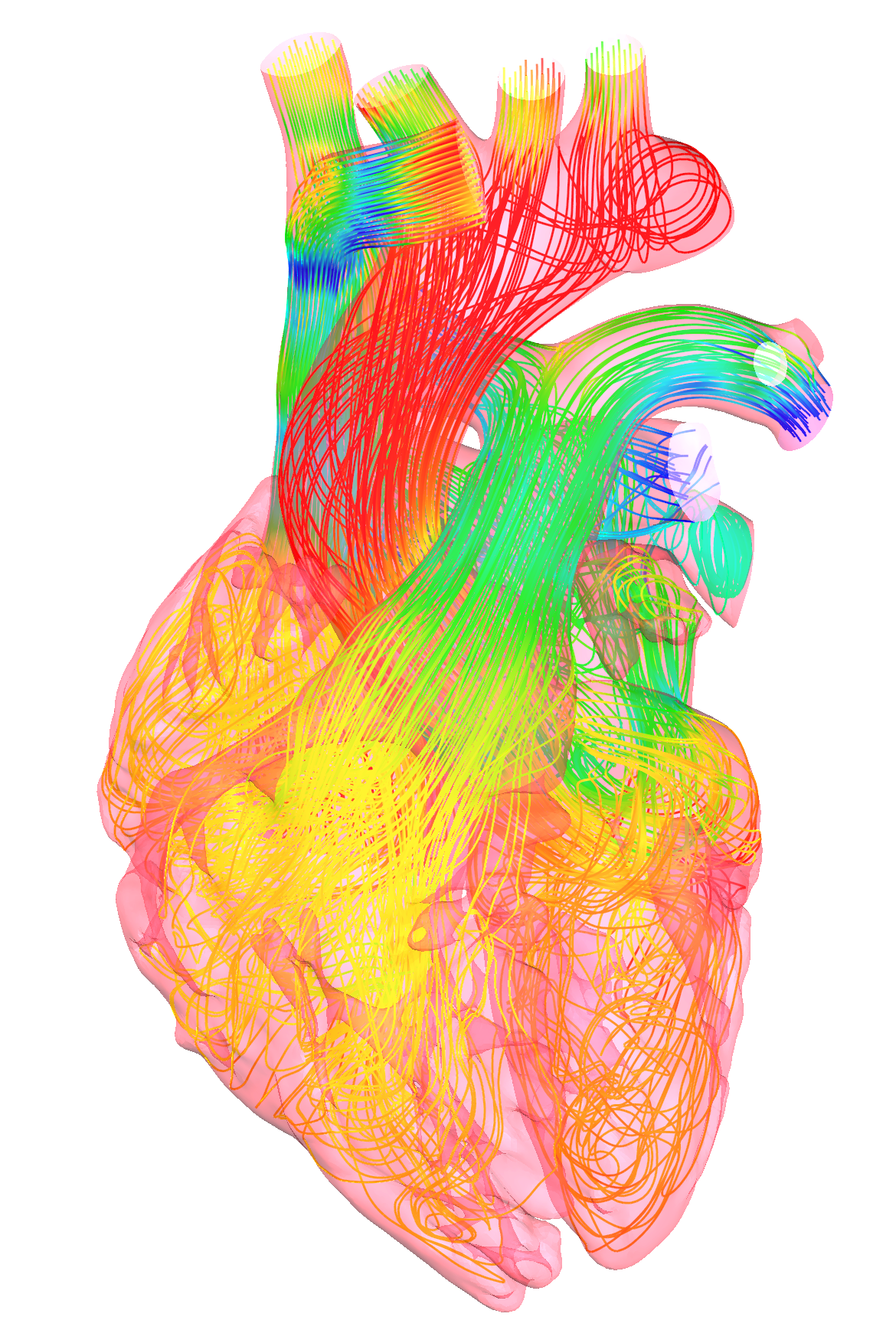
When the radiation model can be used?
If the radiation heat flow is comparable with other heat flow, which is the main heat flow source in the problem (for example, convective heat flow), you have to use a radiation model.
The radiation heat flow can be evaluated based on temperature difference between surrounding environment and the body’s surface using the Stefan-Boltzmann's law:
![]()
The formula above represents the low for the absolutely black body (Plankian radiator). For real bodies you have to multiply the value by emissivity factor.
![]()
- Details

The frequently asked questions at the first acquaintance with FlowVision (before its acquisition and during the using)
- Details
What cells can be called Small cells
In FlowVision uses Cartesian grid that can be automatically locally downscaled. Grid cells intersecting computational domain boundaries and computational subregions are clipped by boundary surfaces.

Fig.1. Splitting cells by geometry surface
After such clipping it is possible that size of new cells will be in many times smaller than initial cell:
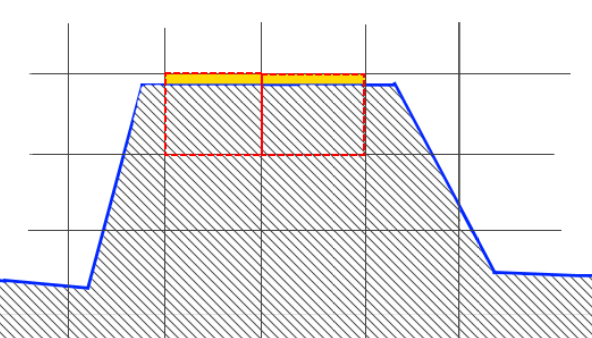
Fig. 2. Small cells
- Details
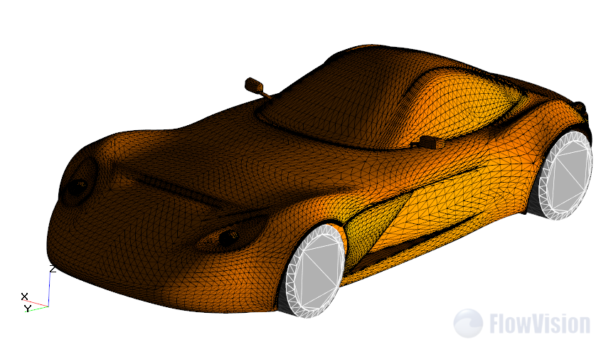
Most prevalent formats of 3D models for FlowVision are STL and VRML. Most of CAD allow to export 3D models to STL and VRML. SolidWorks also allows it.
In this article I will show what parameters of export in SolidWorks will be useful and allow achieving good accuracy of triangulation.
- Details
It is very short article about post-processing in FlowVision. Just main idea which allow you quickly build several ColoredFD pictures.
- Details
Too quick changing of variable can give divergence or make convergence worse, because fast changes will give large gradients of physical variables.
For example, in tasks about turbines and compressors we have rotor which has large velocity of rotation. When we start simulation we can’t specify initial velocity for gas between blades of rotor, because structure of flow too complex. It means that during first time step we will have quick changes of velocity from zero (initial velocity of gas) to some large velocity of blades.
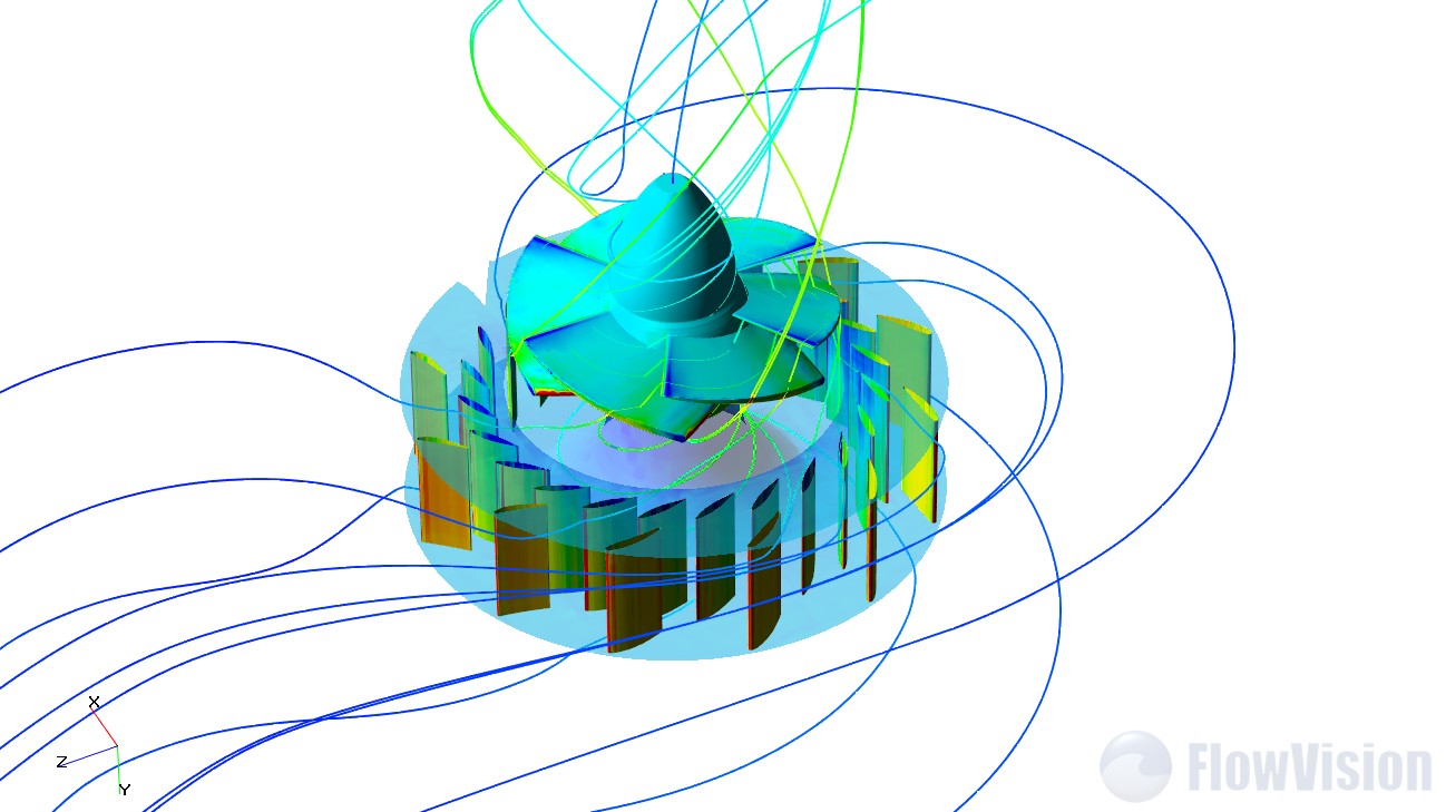
If we will solve this task for incompressible liquid, we will have divergence. It is possible to make convergence better if we will exclude too quick changes, for example, we can change speed of rotation smoothly from zero.
FlowVision allow to specify very complex equations for any user’s variables. Below you will find some formula template which useful to use every time when you need specify some smooth changing of variable.
- Details
In this article you will read about parallelization in FlowVision. It is necessary to understand several features, if you want to get a maximum from advantages of parallel simulations.
- Why is not possible to accelerate simulation infinitely?
- What is role of count of computational and initial cells in parallel simulations?
- How to be faster?
- What hardware is necessary to prefer?
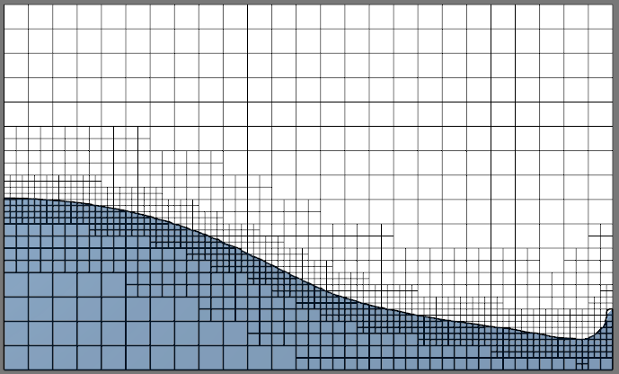
How parallelization works. Computational grid decomposition
When you start simulation, FlowVision first of all will build computational grid and split it for several parts. After this FlowVision will redistribute parts of computational grid between processors. On picture below you can see result of splitting of computational grid for 4 processors:
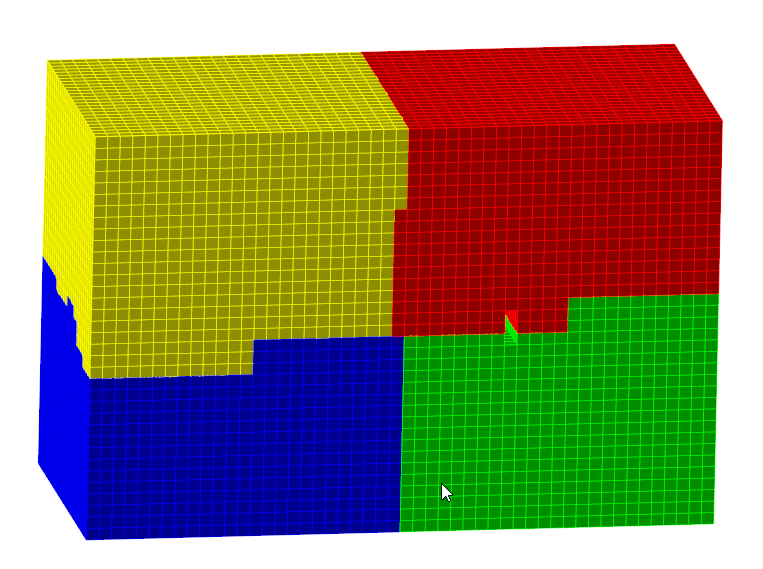
On each processor will be run one copy of Solver which will solve own part of computational grid.
- Details
When doing numerical hydrodynamic simulations, you certainly encounter insufficient accuracy of the obtained results. There can be many causes for this; one of the most typical causes is insufficient resolution by the computational grid.
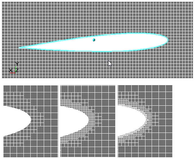
The process of looking for the minimal computational grid, which provides a good numerical simulation of the task (or class of tasks), is known as research of the grid convergence.
This article considers the following aspects:
- What is the grid convergence and why it should be provided
- Best practices of the grid convergence researches
- What happens, if users neglect the grid convergence researches or do not bring them to a successful conclusion?
- What is to be done, if the convergence cannot be obtained because of lack of the computational resources, but we really wish to obtain the results?
- Details
We use QT, Microsoft MFC and OpenGL to give you comfortable tools for pre and post-processing.