In this article you will read about parallelization in FlowVision. It is necessary to understand several features, if you want to get a maximum from advantages of parallel simulations.
- Why is not possible to accelerate simulation infinitely?
- What is role of count of computational and initial cells in parallel simulations?
- How to be faster?
- What hardware is necessary to prefer?
How parallelization works. Computational grid decomposition
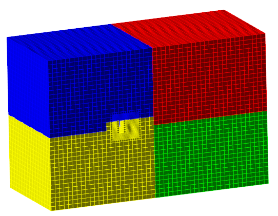
When you start simulation, FlowVision first of all will build computational grid and split it for several parts. After this FlowVision will redistribute parts of computational grid between processors. On picture below you can see result of splitting of computational grid for 4 processors:
On each processor will be run one copy of Solver which will solve own part of computational grid.
Why is not possible to accelerate infinitely. Data exchanging between processors
But when each Solver will solve flows (heat flow, flow of mass and etc.) in cells, sometime it will need to know data from neighbor parts of grid which located on other processors. It means that Solver will request data from other processor. But this exchange of data is very slow process. To ask data in RAM is faster than to ask data from RAM on other node of cluster through the network.
If we want to minimize exchanges, we need to minimize area of borders between processors. FlowVision uses special algorithms for this.
N.B. For constant count of cells there is next effect: the more count of processors the larger losses for exchange between processors. It is possible that increasing of number of processors will give deceleration instead of acceleration. This effect is possible to see on next plot:
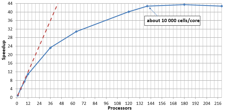
After 180 processors simulation will be decelerated.
It is important to remember that the less count of cells per processor the larger exchange losses (in condition of same total count of cells). Usually optimal count of cells is about 10 000 – 40 000 per core. If you will try to use less count of cells, it is possible that simulation will be slower than in case of less count of processors.
What is scalability?
Plot which shown above is an illustration of scalability. Scalability shows how increasing of number of processors (or cores) will accelerate simulation. Scalability it is not only property of CFD software. Scalability depends from hardware, software and from features of CFD problem and grid.
Ideal scalability is a straight line. It means that increasing of processors in 100 times will give acceleration in 100 times. Unfortunately, in reality it is not possible.
Irregular mesh and scalability
Scalability depends from many factors. Not only from count of cells and hardware. One of important factor is a how computational grid will be built.
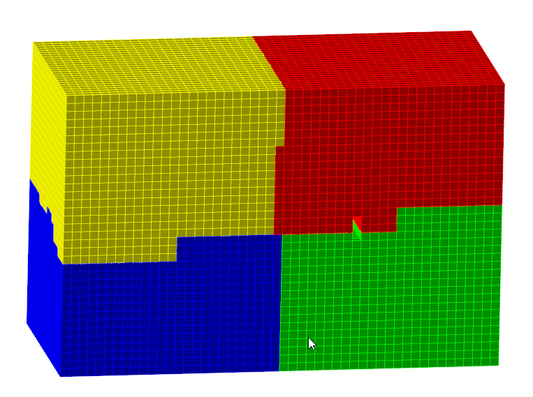
On the picture below you can see result of local adaptation (second level in the volume). You can see that “yellow” processor has many adapted cells. Other processors have less count of cells. It means that yellow will continue simulation when green, red and blue processors finished calculations. It is illustration of misbalance of calculations.
FlowVision’s algorithms try to rebuild such computational grid and make decomposition more balanced.
But it is too hard task if:
- Level of adaptation larger then 4
- Count of initial cells is too small in relation to count of computational cells
- There are many cells which are not computational (vacuum, cells in volume of moving bodies)
These problems can be solved (or solved partly) with Dynamic balancing.
Bottleneck. How hardware influent to scalability
Data exchanging between processors occurs through the RAM. Each thread on each core also store most part of data in the RAM. Each process from each core go to the RAM for new portion of data for calculation. All cores of one processor uses one memory bus.
If count of cores too large we will have bottleneck effect:
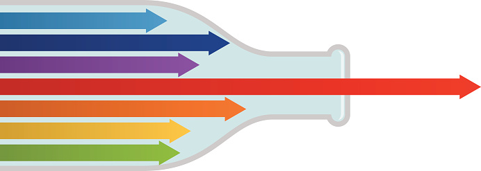
That is why parameters of RAM is more important than parameters of CPU when we talk about CFD simulations. When you choose hardware, you should prefer larger speed of RAM and more count of RAM channels.
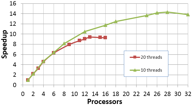
Bottleneck effect also is a reason of effect when using of 80% of cores of one processor will give more large speed then using of 100% of cores. That is why large count of cores in processor is not every time good.
About Hyper Threading
Hyper-threading (HT) is technology, which allows to employ on processor twice much threads than number of physical cores. This technology sometimes allows to achieve better computational performance (up to 30 %). Usually this speedup is possible for computational tasks which have relatively small amount of cells and when computations performed on single personal computer. When a significant number of processors are employed (e.g. cluster, HPC), using HT technology increase of quantity of exchanges with RAM and therefore bottleneck effect may be aggravated. As a result it may lead to decrease of calculation performance.
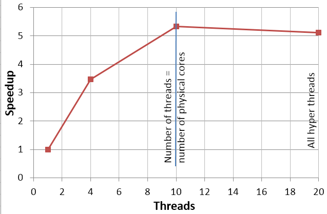
5.2 mil of cells, 8 processors
By the reason mentioned above on those HPCs, which is generally prepared for CFD computations, HT option usually disabled. It may allow to increase the computational performance and scalability limit (curve upper point).
In any case, for exact computational task and exact computational recourses configuration, it is better to try at once, if HT employing have positive or negative effect.
Shortly
When you run parallel simulation you need remember that:
- Optimal count of computational cells per core is about 10 000 – 40 000. You can use more cells, but not less
- Try to use not more than 3-4 levels of adaptation. If you need decrease size of cell, decrease initial grid. Yes, you will have a little bit more number of cells, but scalability will be better
- When you use local adaptation with level> 3 or > 4 , or when you have VOF with vacuum or when you have adaptation over surface of moving body, you can increase scalability with Dynamic balancer.