When doing numerical hydrodynamic simulations, you certainly encounter insufficient accuracy of the obtained results. There can be many causes for this; one of the most typical causes is insufficient resolution by the computational grid.
The process of looking for the minimal computational grid, which provides a good numerical simulation of the task (or class of tasks), is known as research of the grid convergence.
This article considers the following aspects:
- What is the grid convergence and why it should be provided
- Best practices of the grid convergence researches
- What happens, if users neglect the grid convergence researches or do not bring them to a successful conclusion?
- What is to be done, if the convergence cannot be obtained because of lack of the computational resources, but we really wish to obtain the results?
What is the grid convergence? Why it is such important?
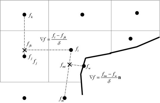
The method of finite volumes, which is used in FlowVision, is based on approximation of the computational domain by finite volumes of computational cells. The whole computational domain is split into boxes (and into polyhedral cells near boundary conditions). Then the program computes for physical variables flows, which flow in and out through each facet of every cell.
Figure 1. Approximation of a variable’s gradient on facets of a boundary cell.
The less is the size of the finite volumes (computational cells) relatively to the size of the whole computational domain, the higher is the resolution of the computational domain. This is similar to the resolution of the computer’s monitor: the higher is the resolution the better details of a picture are displayed.
When physical processes are simulated, it is always necessary to understand which feature of the process is essential, critical for the problem, understand which feature has the most influence on the result. Just this feature (detail of the design, vortex, heat source, velocity profile near a wall) must be primarily resolved by the computational grid.
For example, when simulating of external flow around an airplane, it is quite acceptable to neglect geometry of rivets. Resolution of each rivet by the computational grid is inappropriately because disturbance of flow caused by a rivet is negligible comparing to those pressure gradients, which are generated, for example, by a flap.
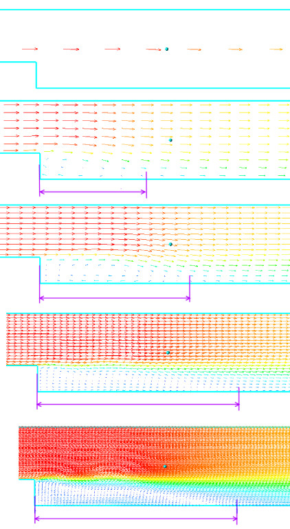
Look at the first illustration of Figure 2 the extreme case: only one cell, which fills the whole diameter of the channel, does not allow the program to form any vortices. When the grid is coarse, you will see the vortex after the backward-facing step, but it will be substantially shorter than the vortex, which you will see when using a high resolution grid. This is because the vortex has not been well resolved by height and it is quickly pressed by the main flow until it evolves into an elongated shadow zone after the step.
Figure 2. Patterns of flow after a backward-facing step were formed at various resolutions of the computational grid. From up to down the resolution changes from 1 to 240 cells along the vertical.
But even when you well understand, which a feature of the simulated physical process needs good spatial resolution, you cannot say definitely, what resolution is sufficient. So a numerical simulation requires a research of the grid convergence.
Approaches to the grid convergence research
In general, the grid convergence research is the research of dependency of the solution on the spatial resolution, which is done by the computational grid.
Steps of the grid convergence research:
- Selection of the mathematical model: At this step it is necessary to correctly select the set of the solved mathematical equations, which completely describe the key physical processes that take place in the simulated arrangement.
- Selection of the character parameters: Here it is necessary to define, which parameters of the arrangement are the key ones, which show the correctness of the received solution. The same parameters are also usually used for determining the moment of the convergence of the stationary solution. For example, for simulation of the fluid’s flow through channels, the most key value can be the pressure drop or the flow rate; for the heat transfer simulations the temperature is to be added to the character parameters. For simulation of the external flow the most interesting parameters can be the lift force and the drag force.
- Simplification of the computational task: Often the grid convergence research can be done on a partial setting up a problem. You should take a part of the simulated arrangement with the most important physical process. For example, for a flow in a channel or external flow around a 3D wing, it is useful to come over to a 2-dimensional setting. The grid, which is found for a 2-dimensional setting, will almost certainly be applicable for a 3-dimensional setting. If necessary, you can test this by making a computation in a 3-dimensional setting on two grids. Use of simplified problem settings allows you to reduce, in several orders, consumption of time and processor resources during researches of the grid convergence.
- Selection of the initial computational grid: The convergence research can be done by many methods, using a grid refinement or an adaptation. For adaptation, you should remember that use of high adaptation levels decrease the multiprocessor scalability of the simulation. Do not use the adaptation level exceeding 5. What is to be the initial size of cells? As an initial point, you can use the following recommendation: a) use at least 4 cells (or, better, use 8-10 cells) at the characteristic dimension of the task (which is, for example, the diameter of an aperture, height of a step, width of a channel, or diameter of a vortex); b) for most of the external flow simulations, you should begin from Y+ that doesn’t exceed 1000 … 10000; c) when you do not use wall functions, (i.e. when resolving the wall layer by the computational grid), begin from Y+ as of 1 ... 2.
- Simulation with sequential refining the computational grid: Depending on complexity of the simulation, you can use different strategies:
- To refine the computational grid, use adaptation over surface a surface or in the volume. This method allows you to use the previously computed solution a good initial approximation for a computation on the new grid. Another advantage of this method is efficient refining of the grid: the grid is only refined in areas, which are the most interesting to the engineer.
- Refine the grid by rebuilding the initial grid. This method has two disadvantages: dimension of the simulation will be higher, because the adaptation is applied in the whole computed volume but not some specific areas; the computation each time has to be started from its beginning. This method is mostly used for 2D computations, because their duration of the computation is only several minutes or hours. The major advantage of this method is refinement of the whole computational volume, that exclude possible mistakes of an engineer, who hadn’t took into account some specific process beyond the area of adaptation (beyond the zone of research the solution depending on the cell size).
- Analysis of the obtained results: After finishing a set of computations made with various grid resolutions, you have to plot how the character parameters (that were defined on the step 2) depend on the size of grid cells. The Y axis on such plots is used for a character parameter, while the X axis is used for the cell size, or for Y+, or for the adaptation level. We can say about receiving the grid convergence when the plot approaches an asymptote, i.e. when the further refining of the grid doesn’t cause a substantial change of the character (control) parameters.
- Reducing the computational grid: As a result of the grid convergence researches, especially when you refine the grid using the method of rebuilding the initial grid, a computational grid will be found, which gives good results but might be a not-optimal. I.e. the found computational grid might be excessive, for example, it might resolve the part of the computational domain, where nothing interesting occurs: there are no high gradients of physical values, no vortices and no geometrical specific details. This part of the computational domain is so locates in the zone of high resolution by some unassignable cause or because of lack of careful analysis for building the computational grid. At this step you can reduce the computational grid in such «calm» locations, testing each time that coercing the grid does not affect the results. The other method of reducing the number of computational cells is applying an adaptation to the solution.
- Modifying the grid with taking into account the full setting of the problem: At this step you can check that the grid, which has been transferred to a 3D setting of the problem from a 2D setting, is also optimal. I.e. this means that its further refining when the cells reduce twice doesn’t cause a substantial improving the results. This is only one calculation but it can prevent errors. Also it might be necessary an additional resolution of geometry elements, which were absent in the 2D setting but might affect the computation.
Step-by-step example of grid convergence investigation
External flow around a 3D airplane’s wing with the Mach number M=0.6 is simulated.
Step 1. Selection of the mathematical model
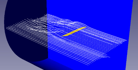
Figure 3. The flow pattern around a wing of finite length in a 3D setting.
When the Mach numbers are large, it is necessary to take into account the compressibility of the gas and its heating. So, it is necessary to calculate not only the Navier-Stokes equations but also equations for energy. Also, the value of the Re number is several orders of magnitude greater than 1500, so it is necessary to use a turbulence model. Because the setting is 3-dimensional, the resolution of the near-wall layer might be inappropriate in an aspect of consuming the computational resources. So we will use wall functions instead of direct resolution of the near-wall layer.
Step 2. Selection of the character parameters
In this simulation the key parameters are the drag coefficient, the lift force coefficient, and the torque coefficient. And it is necessary to examine all the three parameters, because grid convergence of each of them might be obtained at different resolutions of the computational grid.
Step 3. Simplification of the computational task
Length of this wing is finite, but its profile is uniform (the same in all sections). But, anyway, even if the profile isn’t uniform, transition to a 2D setting is reasonable because of economy of resources at the stage of grid convergence researches.
Step 4. Selection of the initial grid
In simulations of external flow, the most interesting are areas of separation (flow breakdown) and areas of shock (if any), the correct resolution of pressure gradients and correct finding the near wall velocity, which substantially define the drag force. Thus, in many aspects, you have to rely on Y+. The wall function can be used when Y+ is greater than 3. This is the lower bound estimate; you can use it as an initial approach. Or you can use as an approach the maximal value of Y+, which is 10000. Or you can select the initial size of cells as a tenth (10%) of the profile’s height.
To evaluate the value of Y+ (at least approximately), you can carry out a computation on a grid with 10 cells per the profile’s height and examine the average value of Y+. When such grid is refined twice, Y+ will reduce about twice.
Step 5. Simulation with sequential refining the computational grid
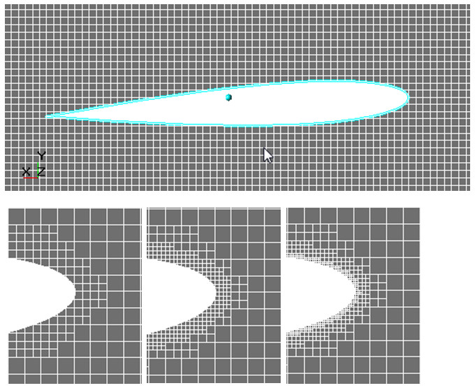
As it was said, the most significant goal of the grid generation in this simulation is good resolution of gradients near the surface of the profile. So we chose the method of refining the surface using a surface adaptation. Several computations have been carried out with successive increasing the level of adaptation.
Figure 4. Evolution of the computational grid during the grid convergence research.
Step 6. Analysis of the obtained results
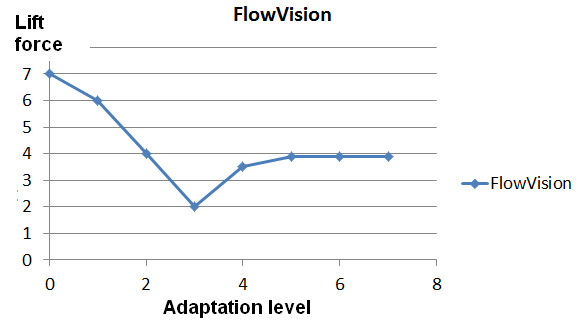
According to the results of the research, the following plot has been obtained:
Figure 5. Dependency of the lift force on the adaptation level by surface
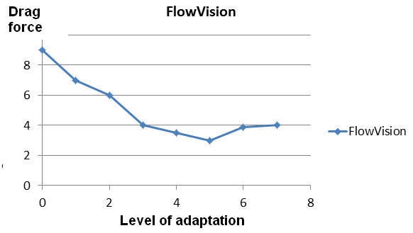
As you see, refining the grid after the 5th adaptation level has a little influence on the lift force, so you can stop on cell size of the 5th level. But when you look at the similar plot for the drag force, you will see that the convergence by this force is reached on smaller grids:
Figure 6. Dependency of the grid force on the adaptation level by surface.
So you have to select the cell size (near the surface) that corresponds to the 6th adaptation level.
Step 7. Reducing the computational grid
In this research the computational grid has been built in several layers for each adaptation level to provide a smooth transition from one adaptation level to another and for careful resolution of value gradients directed normally to the surface.
May be you have selected an excessive number of layers and it is possible to save the grid if you reduce the number of layers on each adaptation level. For this, a computation has been done with the 6th adaptation level and less number of layers per level. Also a computation has been done with much number of layers to make sure that number of layers is sufficient:
Figure 7. Investigation of the influence the number of adaptation layers on the drag force (at the 6th adaptation level).
As you see, reducing the number of layers affects negatively on the results, while increasing of this number changes the results insufficiently. So it does not seem possible to reduce the number of cells - the grid convergence research gave the optimal computational grid at once.
Step 8. Modifying the grid with taking into account the full problem’s setting
At transition to the 3D setting the following specifics have been taken into account:
- A volume adaptation around the side edge of the wing is required to take into account the edge effects of the finite-length wing.
- Use of a high adaptation level (over the 4th level) extremely negatively affects the quality of parallelization of the computation. This is the reason why the initial grid has been refined fourfold to transfer from the 6th adaptation level to the 4th level. Also, for better scalability, the dynamic balance of the grid has been enabled.
Aspects of the computational grid requiring your attention
- At each adaptation level try to use at least 4 layers (and better 8 layers or more). The smooth transition between grids with cells of different sizes provides more accurate and correct solutions.
- In areas of non-zero gradients of physical values and in areas where vortices locate, it is necessary to use cells, which forms are close to cubes. Use of elongated cells in areas where the flow isn’t parallel to the cell faces affects negatively on the accuracy and quality of the solution.
- Do not apply too high adaptation levels, this affects negatively on ability to speed up the computation using multiprocessor system
- When working with turbulence models, watch the prevailing (by area of the surface) value of Y+. Different turbulence models, with wall functions and without them, have limited domains of applicability.
What happens if you do not carry out the grid convergence researches or do not finish them?
Let’s see an example when a user does not carry out the grid convergence research but relies on the experimental results only.
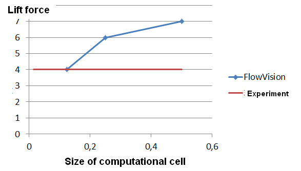
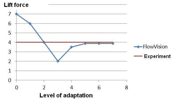
Suppose that an engineer, who simulates an external flow around a wing profile with an attack angle of 3 degrees, tries to refine the computational grid until the lift force be equal to the experimental results, see Figure 8.
Figure 8. Dependency of the lift force on the size of cells. The research has been carried out only up to a point of intersection with the line of experimental values.
The ideal match to the experiment was reached for cell size as of 0.125. Then the engineer decided that the grid convergence has been reached and it became possible to start the simulation of the flow at various attack angles. The obtained results are presented on the illustration below:
Figure 9. Dependency of the lift force on the attack angle in a simulation with unreached grid convergence.
As you see, that at the attack angle of 3 degrees we also have a wonderful coincidence with the experiment, but at all other points the result might be even not complying with the physics of the process.
This situation is also possible in cases when the grid convergence has been was stopped because of the lack of computational resources or time but not based on the nature of the applied numerical methods.
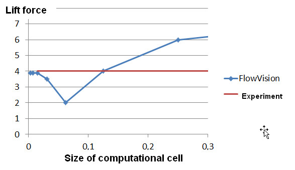
And what would be, if the engineer did not stop the research of the grid convergence and made sure that the convergence had been really reached?
Figure 10. Dependency of the lift force on the size of cells. The research was continued until it was completely and correctly finished.
The same results built for adaptation level over the profile’s surface but not the cell size:
Figure 11. Dependency of the lift force on the adaptation level. The research was continued until it was completely and correctly finished.
As you can see on the illustration above, the further refining the grid causes, at first, causes movement the line away from the value of the experimental result, and then, only the higher adaptation levels, cause asymptotical approach to the experimental result.
But why the solution with the cell size of 0.125m gave such a good correspondence to the experiment? The answer is very simple: this is an accidental coincidence. There are too many chances that two curves intersect somewhere.
Now the engineer is sure that the grid convergence at the attack angle of 3 degrees has been reached. But results of simulation in the whole range of attack angles are disappointing:
Figure 12. Dependency of the lift force on the attack angle for the computational grid, obtained after a correct grid convergence research done for the attack angle as of 3 degrees.
Generally the matching to the experiment is excellent, but when the attack angles are high, FlowVision’s results do not match even the engineer’s knowledge, not the experiment only.
This is because of substantial change of physics of the process at high. The grid convergence research has been done for a small attack angle, for an unseparated flow. When the attack angle is high, a flow separation occurs, and vortices with high pressure gradients appear that cannot be resolved by the grid, which ideally suit to an unseparated flow.
So it is necessary to take into account specifics of various operation modes of the simulated arrangement and, when required, carry out separate researches of the grid convergence. Of course, you might select only several character ranges and do not carry out the researches for each operation mode.
What should you do if you cannot reach the grid convergence because of lack of the computational resources, but you really need the results?
When you simulate complex arrangements, in which it is necessary to take into account the processes that substantially differ in geometrical scale, the grid convergence is reached on tens or even hundreds of millions computational cells. You organization might just have no sufficient computational resources. What can you do, if the convergence has not been reached while you spent all available random access memory?
Recall the history of the computational fluid dynamics, when computers’ random access memory was measured by kilobytes, not terabytes. How solutions of some very complicated problems have been found?
- A qualitative solution is more important than a quantitative one. Do not try to the precise matching to the experiment. The most important is to provide a qualitatively correct solution, when at any mode of flow we receive the expected result, and change of any parameter will change the solution in an expected way. To check that the qualitative solution is correct, you can make a simulation of the arrangement at various modes of flow and make sure that the received curve on a plot is equidistant to the experimental or theoretical curve.
- Try a 2D setting. Transition to a 2D setting substantially speeds up the computation. Evaluate how important are the details, which can only be taken into account in a 3D setting. Might be, it is possible to neglect them?
- Eat an elephant one bite at a time. Analyze your problem. Might be, you could to split these big and complex problem into several independent subproblems? And can you use solution of each of these subproblems as boundary conditions for another subproblem? The simplest example of this approach: a complex pipeline system (with valves, bends and T-joints) can be split into several sections.
Be careful, your attempts to receive a solution without carrying out a grid convergence research can cause loss of your time or even more negative implications. Also do not forget that the computational fluid dynamics has some more abstractions, which should be checked for their influence on the solution:
- Boundary conditions: what are their types and distances from the object(s)
- Time step: what is the time resolution of key processes?

