- Details
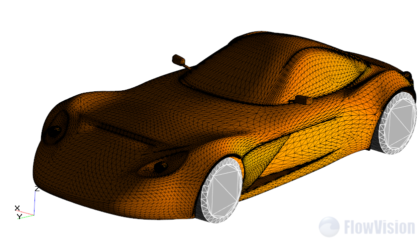
Most prevalent formats of 3D models for FlowVision are STL and VRML. Most of CAD allow to export 3D models to STL and VRML. SolidWorks also allows it.
In this article I will show what parameters of export in SolidWorks will be useful and allow achieving good accuracy of triangulation.
- Details
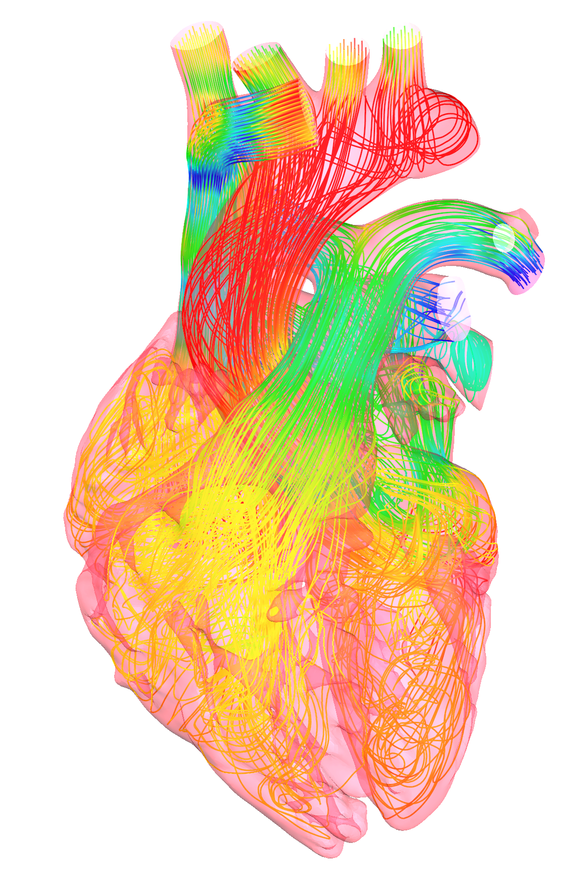
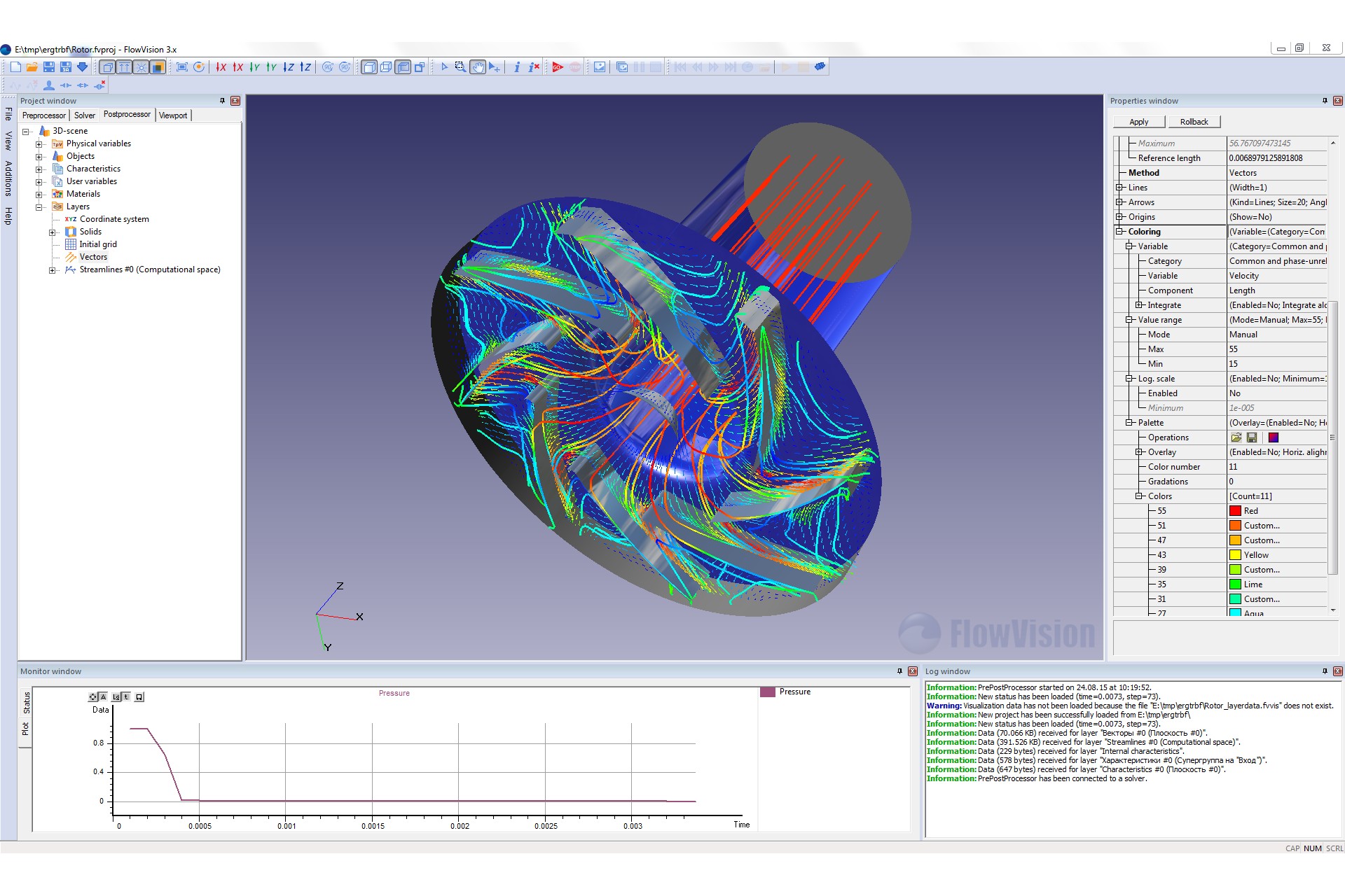
It is very short article about post-processing in FlowVision. Just main idea which allow you quickly build several ColoredFD pictures.
- Details
Too quick changing of variable can give divergence or make convergence worse, because fast changes will give large gradients of physical variables.
For example, in tasks about turbines and compressors we have rotor which has large velocity of rotation. When we start simulation we can’t specify initial velocity for gas between blades of rotor, because structure of flow too complex. It means that during first time step we will have quick changes of velocity from zero (initial velocity of gas) to some large velocity of blades.
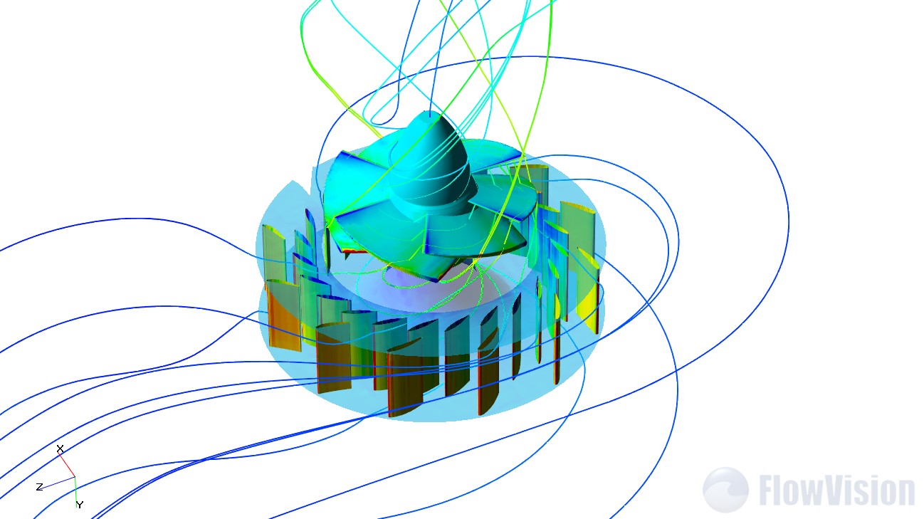
If we will solve this task for incompressible liquid, we will have divergence. It is possible to make convergence better if we will exclude too quick changes, for example, we can change speed of rotation smoothly from zero.
FlowVision allow to specify very complex equations for any user’s variables. Below you will find some formula template which useful to use every time when you need specify some smooth changing of variable.
- Details
In this article you will read about parallelization in FlowVision. It is necessary to understand several features, if you want to get a maximum from advantages of parallel simulations.
- Why is not possible to accelerate simulation infinitely?
- What is role of count of computational and initial cells in parallel simulations?
- How to be faster?
- What hardware is necessary to prefer?
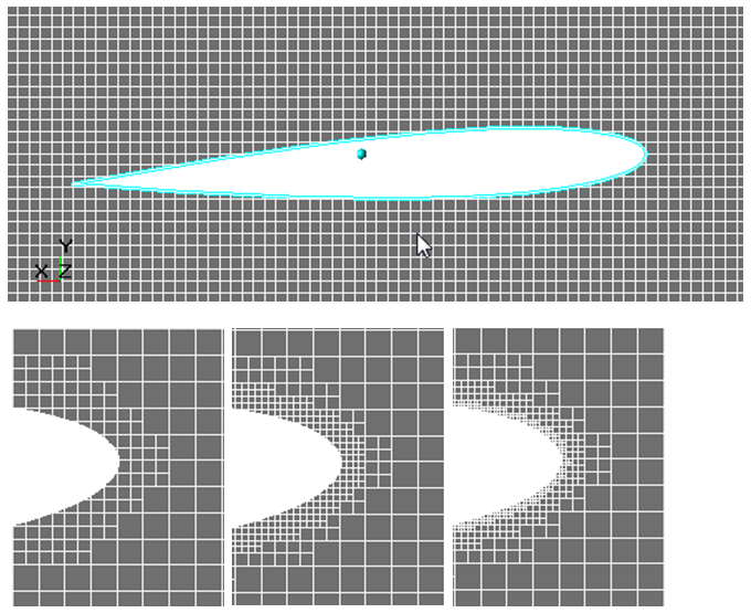
How parallelization works. Computational grid decomposition
When you start simulation, FlowVision first of all will build computational grid and split it for several parts. After this FlowVision will redistribute parts of computational grid between processors. On picture below you can see result of splitting of computational grid for 4 processors:
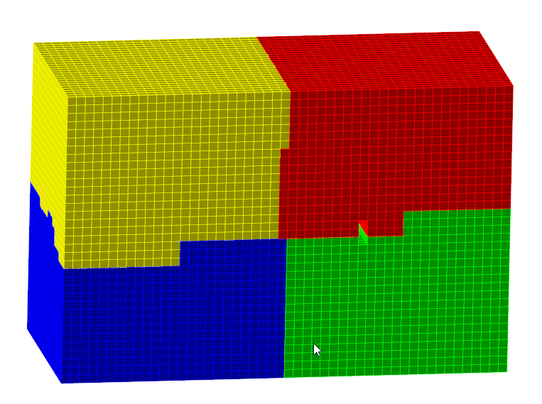
On each processor will be run one copy of Solver which will solve own part of computational grid.
- Details
When doing numerical hydrodynamic simulations, you certainly encounter insufficient accuracy of the obtained results. There can be many causes for this; one of the most typical causes is insufficient resolution by the computational grid.
The process of looking for the minimal computational grid, which provides a good numerical simulation of the task (or class of tasks), is known as research of the grid convergence.
This article considers the following aspects:
- What is the grid convergence and why it should be provided
- Best practices of the grid convergence researches
- What happens, if users neglect the grid convergence researches or do not bring them to a successful conclusion?
- What is to be done, if the convergence cannot be obtained because of lack of the computational resources, but we really wish to obtain the results?
- Details
We use QT, Microsoft MFC and OpenGL to give you comfortable tools for pre and post-processing.