- Details
You have started a simulation of physical processes in Flow Vision by yourself, but the calculation always breaks down. Or the calculation runs, but the results do not correspond to physics. Is it familiar to you? Here is the quintessence of the experience from technical support and the training department staff. It`s a guide on what to do if your calculation breaks down.
- Details
To obtain the exact solution in numerical simulation, the reference values should be set correctly. Find out from this article how to set the reference values and how they affect the accuracy of the solution. We also examined two cases that our users usually face. Forewarned is forearmed.
- Details
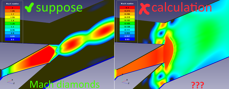
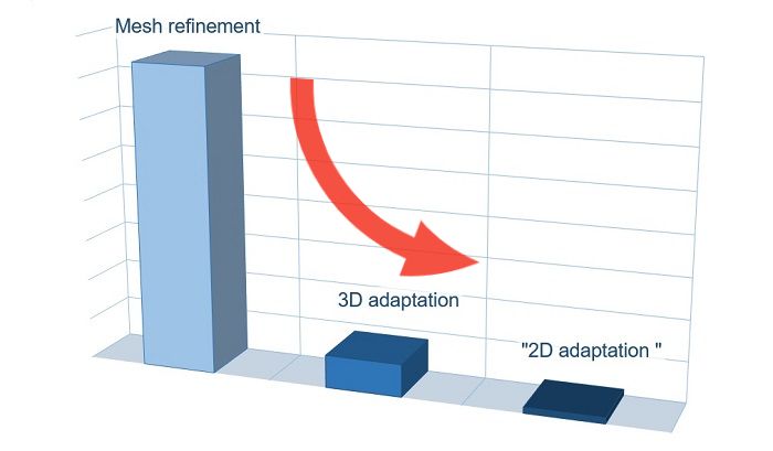
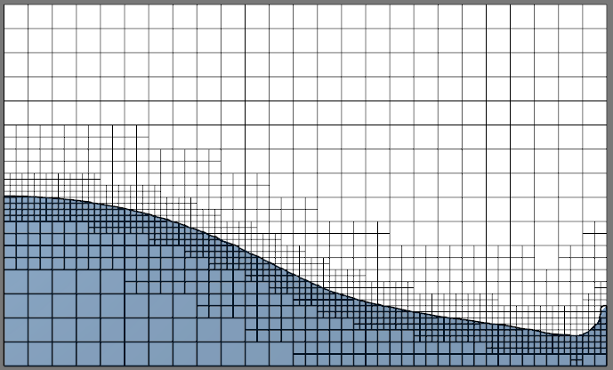
Today we will talk about minimization of the computational mesh in a two-dimensional calculation. In general, FlowVision is a three-dimensional CFD software. But the 3D calculation becomes 2D if there is only one calculation cell in one direction. Unfortunately, two-dimensionality disappears when adaptation is enabled. User of FlowVision from JIHT figured out this issue.

- Details
Sometimes the situations appear, when the co-simulation may be interrupted for a number of reasons:
1. Lack of memory (both operational and physical);
2. Restarting the machine on which the calculation has been carried out.
3. The necessity to stop the calculation for project modification.
If the simulation is carried out only in FlowVision, the problem is easily solved by continuing the simulation from the last save. In the case of a joint simulation, the procedure is more complicated.
- Details
FlowVision uses floating type of license. It means:
- The license is installed and attached to one computer and can’t be transferred or registered on another computer;
- But users can work with FlowVision on any computer and they can even constantly change their working computer. FlowVision will request a license from the computer on which the license was registered.
- On one computer it’s possible to register many licenses for different users. It allows to avoid blocking license, for example, of the user of neighboring department.
- You can also register one general license, for example, with a large number of cores and allow users to compete for licenses :) This allows you to run the calculation on the maximum number of cores if necessary.
Thus it is convenient for a company to allocate a server for registering and storing a license instead of, for example, a laptop.
- Details
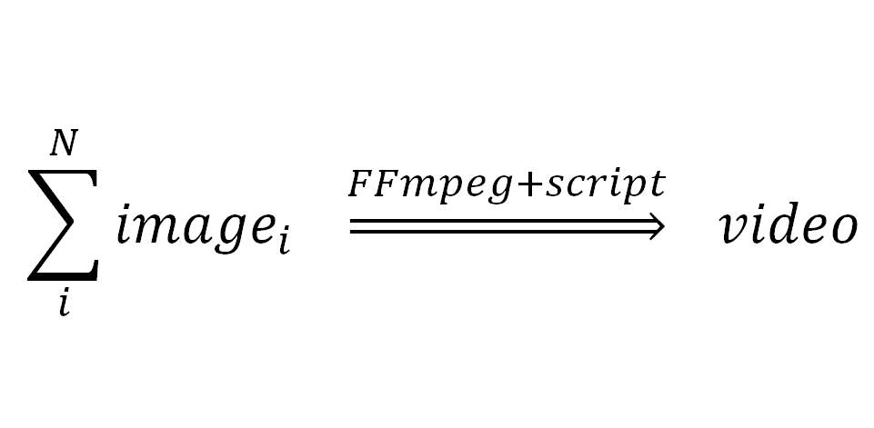
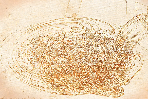
When modeling a physical phenomenon, the most informative way of visualization is video.
In this article, we will describe how to turn a sequence of images into a video clip.
- Details
This article will be useful for the beginners who want to learn more about the turbulent flow and pitfalls encountered during its modeling. We'll go through:
- Details
FlowVision 3.11.01 obtained a new connector for linking to Abaqus. The new connector calls Abaqus CSE. This connector expands possibilities of direct coupling connector and has following advantages:
- More flex settings of co-simulation;
- Easier launching at cluster machines;
- Introducing of additional programs into co-simulation;
- Interaction with newest version of SIMULIA Abaqus.
Such advantages are realizing by Abaqus module: Abaqus CSE Director. But such approach has his own disadvantages:
- Abaqus CSE Director requires configuration file for his work;
- Complex launching of Abaqus which is not supporting by MPM-Agent of current FV version.
The problem of file generation was resolved. FlowVision creating file by user request. As input data FlowVision use Abaqus project which needed for connector creating.
Analysis launching by MPM-Agent has problems with commands which are transferring to Abaqus: are separated launching of Abaqus CSE Director and separated launching of project.
Script was created for resolving this problem and making launching of Abaqus more simple. This script taking data from FlowVision project and allows launching both type of connectors: Direct coupling and Co-simulation Engine.
Script as for Windows OS, as for Linux OS is attached to this paper for using.
- Details
There are many improvements in new version of FlowVision 31001. They significantly concern to functionality of adjusting and editing of computational grid such as computational grid adaptation, parameters of boundary layer grid etc. The list of main changes in comparison with FlowVision 31001:
- All adaptations and boundary layer grid are specified now in separate section of project tree named “computational grid”
- In project tree active adaptations and boundary layer grid are highlighted by color while inactive adaptations are grey-colored
- Subregions and geometrical objects in PreProcessor with the same settings of computational grid can be grouped to single subsection of project tree. It is not necessary to repeat this settings separately for each item anymore.
- It is possible to adjust number of layers for intermediate adaptation levels (not only for maximal adaptation level as in previous version). It is not necessary to create such grid during several number of solution steps
- New function is “adaptation by condition” which allow to make split of cells according to specified condition (range of values for variables)
These and other most meaningful features are described below.
- Details
When the radiation model can be used?
If the radiation heat flow is comparable with other heat flow, which is the main heat flow source in the problem (for example, convective heat flow), you have to use a radiation model.
The radiation heat flow can be evaluated based on temperature difference between surrounding environment and the body’s surface using the Stefan-Boltzmann's law:
![]()
The formula above represents the low for the absolutely black body (Plankian radiator). For real bodies you have to multiply the value by emissivity factor.
![]()
- Details

The frequently asked questions at the first acquaintance with FlowVision (before its acquisition and during the using)
- Details
What cells can be called Small cells
In FlowVision uses Cartesian grid that can be automatically locally downscaled. Grid cells intersecting computational domain boundaries and computational subregions are clipped by boundary surfaces.

Fig.1. Splitting cells by geometry surface
After such clipping it is possible that size of new cells will be in many times smaller than initial cell:
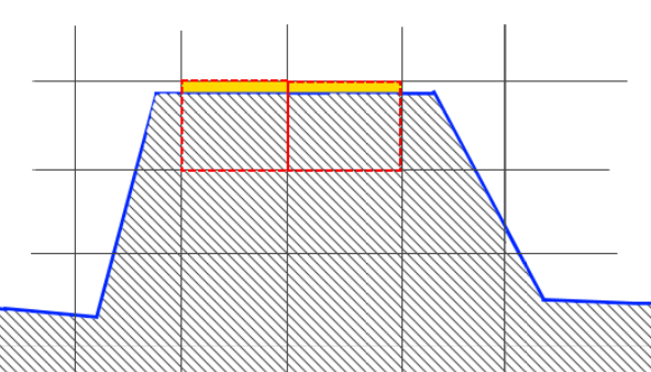
Fig. 2. Small cells