Dispersed flows: step-by-step
Dispersed flows are one of the more extensive and therefore most popular classes of dispersion problems among users. (Problems with disperse decomposition, icing, and coal combustion are also popular, but to a lesser extent). Fogs, aerosols, powders, solid admixtures, suspensions (cement mortar, orange juice) and emulsions (bitumen, milk) - all these substances surround us not only in industry, but also in everyday life. Let's move from theory to practice and add particles to the laminar pipe-flow tutorial. Instead of water flowing through the pipe, let it now be a suspension of sand (SiO2) in water. Here we will go over the most important of them:
- Number of size groups in the spectrum
- Physical processes in the dispersed phase
- Particle cloud drag coefficient
- Nusselt number
- Dispersion settings on BCs
- Multiphase D
- Variables in the Postprocessor
JUST ADD PARTICLES
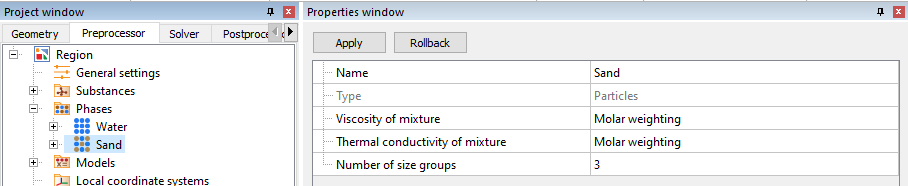
Start modelling dispersed flows by creating a "Particles" phase where you are immediately taken to the key settings: Particles> Number of size groups.
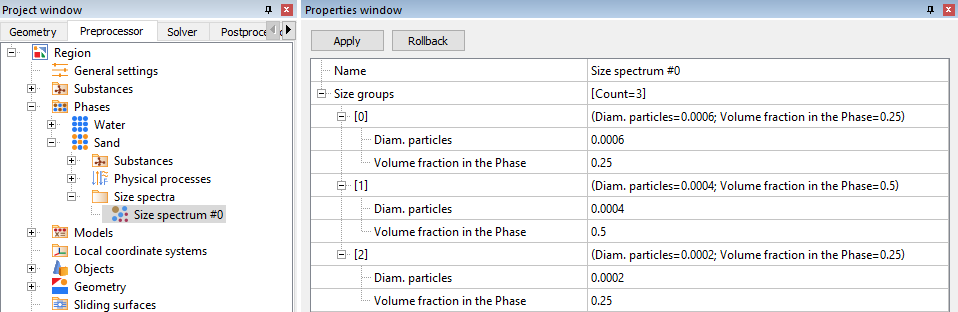
Then create a Size Spectrum, which will consist of three size groups with different diameters. Of course, it is worth keeping in mind that the sum of the volume fractions of all groups = 1.
One phase can contain up to a maximum of 100 different size groups.
It is unlikely that you would need more than this. The limit on the number of groups is linked to the capabilities of computing machines: for each (out of 100!) size groups, there needs to be allocated a certain amount of RAM, which in modern realities is not an unlimited resource.
PHYSICAL PROCESSES
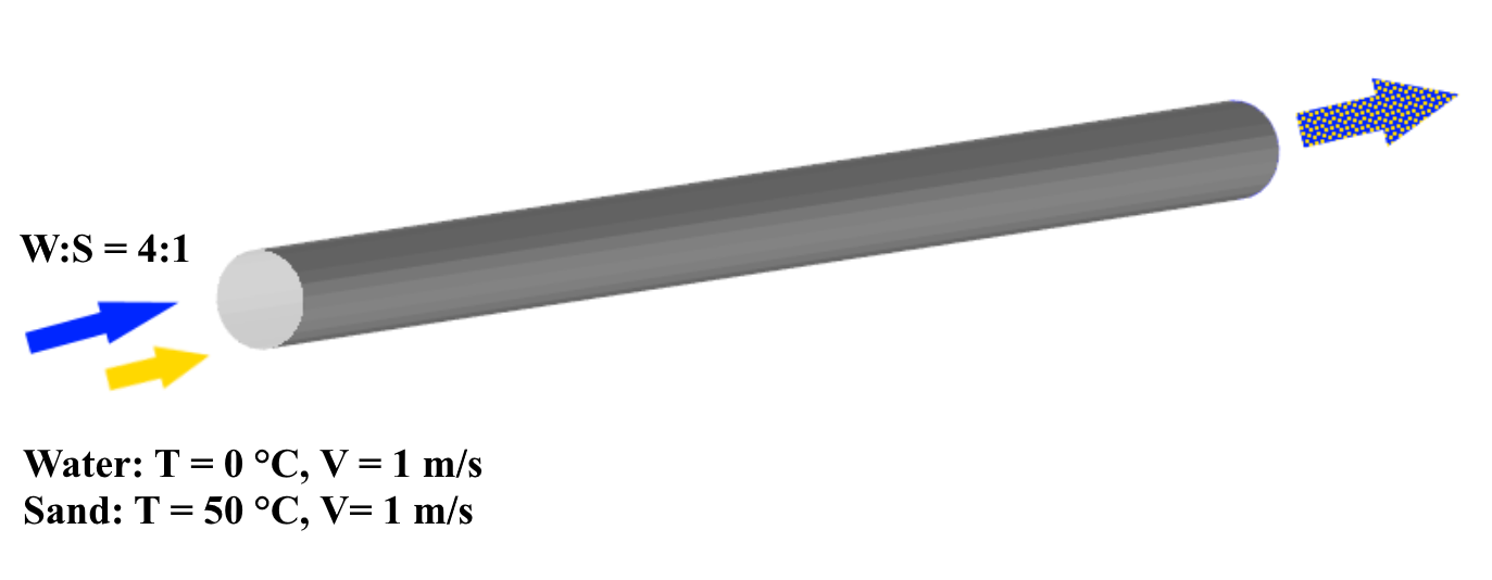
Let's give a more detailed definition of the scenario being simulated. Let hot sand (T = 50°C) and cold water (T = 0°C) enter through the pipe inlet with a ratio of 1:4. Furthermore, let’s assign three distinct groups of sand grains with sizes (d1 < d2 < d3) in a ratio of 1:2:1. This mixture of water and sand, intermixes further as it flows through the pipe and exits at the other end.
 For modelling, we take into account the following processes:
- Heat transfer in the dispersed phase (as part of the heat exchange process between the dispersed medium and the continuous phases) > heat transfer = convection and conduction
- Transfer of particles of different diameters within the dispersed phase > phase transfer = convection and diffusion
- Motion of the particle cloud within the continuous phase > motion
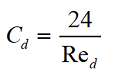
PARTICLE DRAG COEFFICIENT
Model > Phase interaction > Continuum - Particles > Сd
To calculate the drag coefficient of particles, select one of the five models.
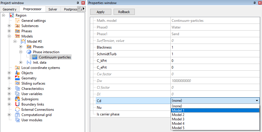
The drag coefficient (Cd) for the dispersion cloud is determined by the environment through which it flows. For a continuous phase (Knudsen number, Kn < 0.001), the focus is typically on the dependence of drag coefficient on Reynolds number, Re.
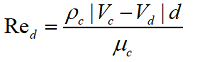 Parameters with index "c" are parameters of the continuous medium, and those with index "d" are parameters of the dispersed medium.
The first scientist to propose that the coefficient of resistance is dependent on the Reynolds number was Sir George Gabriel Stokes. The relationship he derived is in excellent agreement with experimental data for Re <0.1.
- Models 1, 2 are close to Stokes flow, where particles have low velocity relative to the overall flow.
- Models 3, 4 were developed based on the works of (Ergun/Wen and Yu) and (Cheng), respectively, and allow the range of Re numbers of dispersed particles to be expanded up to Re < 3⋅105. These models work well for simulating the spraying of particles within a stationary domain.
- Model 5 is used in bubble modelling. Read more about this process in the next article on dispersion.
NUSSELT NUMBER
Model > Phase interaction > Continuum - Particles > Nu
To calculate the Nusselt number for the particles, select one of the two models.
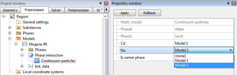
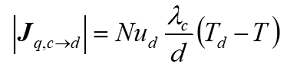
The Nusselt number (Nu) describes the ratio between the convective and conductive heat transfer and is used to determine the heat flux:
- Model 1 is more universal, and is suitable for modelling the joint movement of particles in a stream, and the movement of particles in a stationary environment.
- Model 2 is split into two expressions for calculations at low and high Re numbers.
DISPERSION SETTINGS AT BOUNDARY CONDITIONS
For each of the selected physical processes, it is necessary to define the following properties of the dispersed phase at the boundary conditions:
- Phase volume (Sand)
- Temperatures (disp.) (Sand)
- Velocities (disp.) (Sand)
Inlet (Inlet/Outlet)
At the inlet we set values based on the provided data: we know the values for phase volume (= 1/5 = 0.2), temperature (= 50 when Tref. = 273) and velocity (= 1).
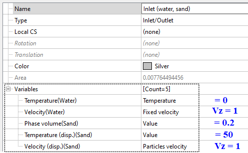
Provided the flow rate of particles over a BC is known, we can set either the volumetric velocity (Vd⋅φd) or the mass velocity (ρd⋅Vd⋅φd).
Outlet (Free outlet)
On the surface corresponding to the physical outlet, set the condition ‘permeable surface’ for all variables related to the dispersed phase. This ensures undisturbed flow for the dispersed phase. The permeable surface condition is analogous to the zero gradient condition for the continuous phase. For water, we also ensure the undisturbed outflow of the medium by setting the pressure value to zero.
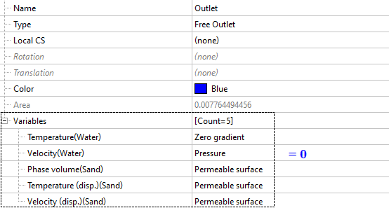
If the outlet flow rate or outlet parameters are known, then you can also set fixed values for the dispersed phase variables at the outlet BC.
Pipe surface (wall)
At the pipe walls, the velocity is described using the condition contact with wall, which you can use to vary the direction in which particles rebound off the wall.
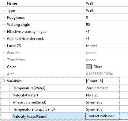
If you are modelling membranes, then FlowVision allows you to assign a permeable wall condition: set the values for phase volume, temperature, and velocity (just like for an inlet BC), and for the continuous phase leave the condition of no flow through the walls.
MULTIPHASE D
Dispersed multiphase settings are located under the Solver tab > Advanced settings.
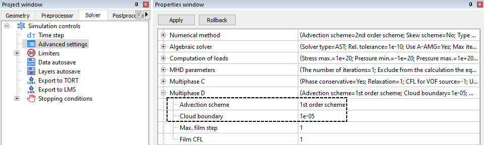
The maximum film step and film CFL are only used when modelling icing. In this sense, Advection Scheme and Cloud Boundary are the more universally used dispersion parameters.
- Empirically, it has been determined that, in the current FlowVision implementation, using 1st order accuracy for the advection scheme leads to a more stable solution.
- The cloud boundary defines the lower limit for the value of the dispersed phase in a cell. If the actual phase value is less than the cloud boundary, then the particles in this cell are excluded from the calculation. By default, the cloud boundary value is 1e-5.
POSTPROCESSING: DISPERSED PHASE VARIABLES
The complete list of dispersed variables is displayed when you select the category Variables of phase “Sand”. Let's consider the ones typically used:
- Concentration [m-3] – the number of particles in a cell
- Phase volume [-] – the share of a cell occupied by the dispersed phase
- Velocity (disp.) [m/s] and Temperature (disp.) [K] relate to the dispersed phase only. The respective variables for the continuous phase are labelled Velocity and Temperature.
The specific size group that particles belong to is shown by the index in the square brackets: [0, 1, or 2]
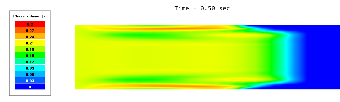
For example, phase volume indicates the total share of the dispersed phase, whereas phase volume [1] indicates the share of only the 1st group of particles (with diameter 0.0004 m). Let’s display the distribution of sand near the pipe inlet. To do this, we use the Variable of phase "Sand" > Phase Volume.