Introduction to Particles
Let's start with the definitions
Dispersed medium – refers to either small particles in a gaseous, liquid or solid aggregate state, or a solid with cavities (pores). Visions of humid sea-side air, sandy beaches and a glass of lemonade evoke thoughts of summer, but are also demonstrative examples of dispersed media. In these examples we can see the key feature of these media - particles do not exist on their own, but rather interact with the continuous phase carrying them:
- water droplets are carried by the air flow
- gas bubbles float in the drink
- water seeps through the sand into the ground
Furthermore, the particles are evenly distributed amongst the molecules of the continuous phase, without entering into a chemical reaction with them.
The interactions of the dispersed and continuous phases form a dispersed multiphase system. Based on the particle size (d), we can distinguish between coarse and fine dispersed systems. And if the particle diameter is similar to the size of the molecules of the carrier medium, then such a system is dubbed a true solution. It is not at all necessary for all particles in a dispersed system to have the same size and shape. On the contrary, they will most likely be completely unlike each other.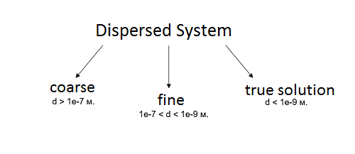 In FlowVision, the assumption is made that the particle size is always much larger than the molecule size. Under the initial and boundary conditions, the user can choose to model either identical particles (which have a specific average diameter), or a spectral distribution of particle sizes.
Dispersion in FlowVision: Particles and Carcass
Depending on the aggregate states of the dispersed and carrier phases, different dispersed systems are formed. All their diversity is displayed in the following table: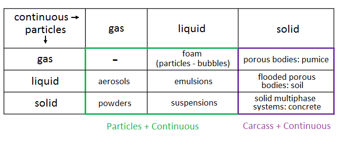 In FlowVision, dispersion in gaseous and liquid media is defined by the interaction of "Particles + Continuous", and flow through a solid porous medium is defined by the interaction "Carcass + Continuous".
So what's the difference?
Conceptually, the phases "Particles" and "Carcass" are similar - within the framework of the Euler method, each can be considered to be a continuum. However, the physics for these two phases are different. The main difference is that the "Carcass" phase is rigid. It follows that the models and relationships applied to particles and rigid bodies are different: the physical process equations for a Carcass do not have a convective term. And anyway, the equations for Motion and Phase Transfer are pretty much irrelevant for a Carcass.
At this stage, let's follow the example set by our developers and split our account of FlowVision’s dispersion capabilities into two parts: Particles and Carcass. From here on the sole focus of the article will be the Particles. The use of a Carcass for modelling heat exchangers, filters, soil and other porous media, will be covered in the third article of this series.
Euler's Method in Particle Modelling
In FlowVision, the particles being considered are combined into a dispersion cloud. Thus, physical processes are not evaluated for each individual particle, but rather for a volume of space, which has the properties of a continuous medium. Therefore, when simulating a multiphase flow, the cloud of particles and the continuous carrier phase interact as interpenetrating continuous media.
However, this approach does not explicitly take into account the collisions of particles with each other and, as a result, there are no stresses inside the cloud. Therefore, it is typical to introduce additional models (e.g. fluidized bed model) in order to account for this interaction of particles with each other within the framework of the Euler method. FlowVision implements a simple repulsion model that introduces an additional term to the particle motion equation. It’s coefficients can be edited within the FlowVision interface.
Why does the dispersion solver use Euler's method?
Another approach to modelling particles in a continuous medium is the Lagrange method. It involves solving a larger number of equations for the modelled particles. Each modelled particle represents a certain (fairly large) number of real particles. The Lagrangian solver records the movement of these model particles from one face to the next for each cell through which the particle trajectory passes. The Lagrangian method had been implemented in the 2nd generation of FlowVision. But as of FlowVision 3.xx.xx it was decided to switch to the Euler method, which requires less computational resources and less RAM. Both methods (Euler and Lagrange) have their advantages and disadvantages. A detailed overview of these can be found in literature on the subject.
What is FlowVision able to simulate using particles?
- Multiphase dispersed flows: aerosols, powders, emulsions, suspensions
- The movement of gas bubbles in a liquid (taking into account the change in size of the bubbles)
- Evaporation of liquid droplets
- Combustion of coal and similar substances that separate into water, coke, and ash
- Jet spraying from a nozzle (taking into account the splitting and merging of drops)
- Surface icing
Limitations
- The current implementation in FlowVision does not support the adding of more than one dispersed phase to a model (i.e. each model is limited to only one Particles or only one Carcass phase).
- FlowVision is not yet able to model the phase transition of a continuous phase changing to a dispersed one.
Aside from limitations, there are also strong capabilities:
- Particles can participate in multiphase VOF interactions: (particles + continuous #1) + continuous #2.
- FlowVision 3.12.02 introduced a model for particle condensation. Condensation modelling is currently in beta testing, so if you encounter any difficulties in applying the model, please contact technical support: support@flowvisioncfd.com.
- Particles are compatible with periodic boundary conditions and sliding surfaces.