The FSI Checklist

To make life a little easier for a beginner in FSI, we have prepared a checklist of steps that are standard to all FSI projects. In reality, this is just the tip of the iceberg, since each project has its own specific characteristics.

What does one need to know in order to run joint calculations?
The answer to this question is not that simple. Let's go through the checklist together and reveal all the subtleties and "secrets" at each step.

The FSI project checklist

Or a brief overview of the main points. In this section, we will examine the basic set of actions required to prepare and launch a joint calculation, namely:

• How to set up an Abaqus project
• How to set up a FlowVision project

Setting up an Abaqus project

You have prepared an Abaqus project and want to perform FSI calculations. But before getting started with the FSI project, it is important to perform a series of steps that will help avoid future mistakes and questions. The steps that need to be performed:

• Check the dimensions of the Abaqus project.
• Launch the Abaqus project for calculation. Make sure the Abaqus project can be launched and runs successfully without FSI (you can just comment out the co-simulation lines if you have already added them).
• Create exchange surface(s).
• Select variables for data transfer (U - displacements, COORD - coordinates - for Abaqus, PRES - pressure, CF - concentrated force for FlowVision).
• Set up co-simulation lines in the .inp file.

Configuring the FlowVision project

To set up a FlowVision project, you need to:

• Check the unit system being used in the project.
• Create an "Imported Object" - import the geometry of the object (objects), which are to be deformed.
• If modeling deformations of an object with a complicated shape, then there is a possibility that its geometry contains self-intersections. If this is this case, FlowVision will not be able to run the project. To check for this: right click on the imported object > check geometry for self-intersections. If FlowVision happens to find self-intersections, then you will need to remake the geometry in line with FlowVision requirements.
• Create a Moving body modifier on the imported object and, if necessary, scale / move / rotate the object via the modifier properties. It is important to correctly place the body in the starting position.
• Create an external connection with the FE-complex.
• If necessary, set heat / load relaxation.
• Edit connection settings: specify the IP address of the computer that will be running the FE-complex and the port over which to connect.
• Run the FV project for calculation without connecting to the FE-complex and make sure that the calculation launches successfully and the results are physically sensible. For this, turn on the "Disable connectors" option when starting the calculation.

Launching an FSI calculation

• Run Abaqus via the command prompt.
• Start the calculation in FV: this can be done via the PrePostProcessor, Terminal, and also via the command prompt, having prepared a command file.
• Having launched your simulation, you can observe the deformation of bodies via the Viewer module.

Configuring the Abaqus project

If you are not creating a fresh Abaqus project, but merely setting one up for connection, then not much is needed at this stage. To set up a project, you will need to know the following:

• How to check dimensions (necessary for the later configuration of the FlowVision project).
• How to create an exchange surface
• Connector type
• How to work with inp-files

Checking project dimensions

For Abaqus and FlowVision to work correctly after connection, they need to be brought to a single measurement system. For FlowVision, that system is SI, and is used for all variables and calculations. By default: lengths are dimensioned in meters, time is in seconds, pressure in Pascals, and force in Newtons.

Abaqus, however, isn’t bound to any specific measurement system. The user chooses which system to work in, and the responsibility for correctly setting parameters (dimensions) lies with them. This means that if the user has created a part in mm, then all further parameters must be specified in the dimension of mm-ton-seconds and their derivatives. For example, material density will need to be specified in tons / mm3.

There are several ways to check which unit system an Abaqus project has been created with:

1. Measure the characteristic length of a part and compare it with that of the real object.
2. Look in material properties and check the value for density. For example, if the it contains powers of -9, then the project has been created in mm, and the density is in tons / mm³.

It follows that if the projects have been created using different systems of measurement, then for a joint calculation to work correctly, they must be brought to a single system. This can be done in one of  two ways:

1. Set all FlowVision values matching the Abaqus system of measurement. This is quite labour intensive - you can easily make a mistake, manually translating all values from one measurement system to another. We do not recommend using this approach.
2. Use scaling factors for geometry, loads, and temperatures.

Creating an exchange surface

To set up the connection between the ABQ and FV projects, you need to select a surface within Abaqus to receive load data from FV and deformation data from ABQ. The exchange of these two sets of data will happen along this surface.

To create an exchange surface, you need to be able to work with geometry in Abaqus. At the very least, you need to be able to create surfaces by selecting parts of the geometry. The Create option in the Assembly module in the Surfaces section will help you here:

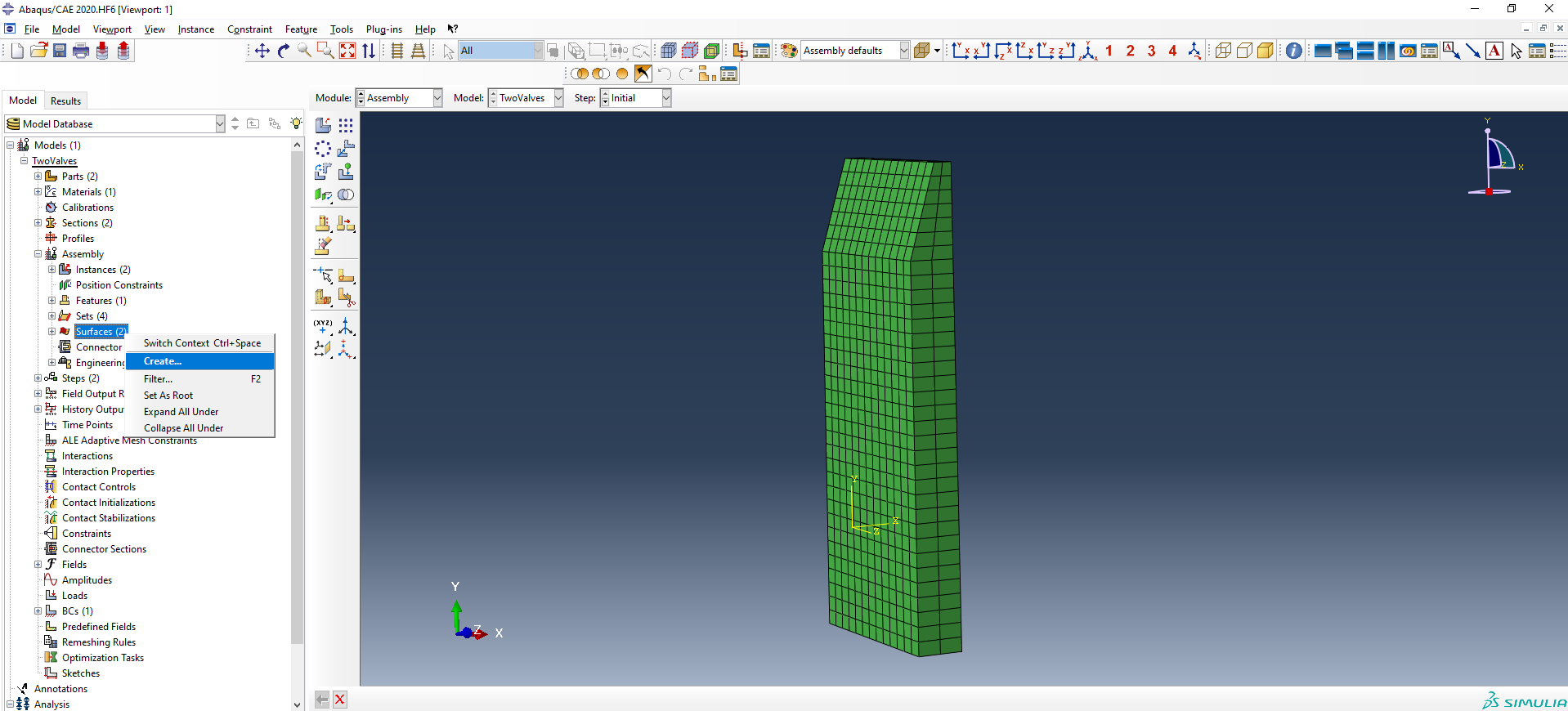
When selecting a surface, you should turn your attention to where and how it is being created. There is a risk that the surface will be created on the inside of a part, on part of a part, or on the inside of an element. This is especially likely when constructing from Shell elements. If you are using them, then when creating the surface, select the correct side of the shell using the Choose a side for the shell or internal faces option. For most FSI projects it is the outer surface that is used to transfer loads. Also, keep in mind that the exchange surface must be closed. More about requirements for exchange surfaces here.

Connector type

Currently, one of two types of connectors can be used to connect to Abaqus:

• Abaqus Direct Coupling
• Abaqus CSE.

The first (Abaqus Direct Coupling) is an outdated connector type that mainly works with older versions of Abaqus (up to and including Abaqus 2016).

The second (Abaqus CSE) is a newer connector that facilitates interaction with later versions of Abaqus (Abaqus CSE - v2017 onwards).

Working with inp files

An inp file is an Abaqus file that contains a description of the entire project in text form. It can be opened with regular notepad or the more advanced Notepad ++ (more convenient).

To work with FSI calculations, it is imperative to learn how to work with inp files. At early stages, you won't need to modify this file much for simple calculations. For example, in one tutorial project, you just need to add co-simulation lines to the end of the file. But for complex projects, more significant changes may be required, for example, manually adding exchange surfaces, or adding / removing boundary or initial conditions.

The co-simulation lines contain the following information:

1. The type of joint calculation - whether the connection uses Direct Coupling or CSE connector.
2. The name of the exchange surface (must be preceded by ASSEMBLY_).
3. The transmitted variables: U = displacements, COORD = coordinates (for Abaqus), PRES = pressure, CF = concentrated force (for FlowVision).
4. Settings for joint calculation, if it is a Direct Coupling connection (e.g. time incrementation = subcycle, time marks = yes)

For more information on co-simulation parameters for various connectors, see the Abaqus documentation.

Creating and configuring the FlowVision project.

To prepare a FlowVision project for FSI, you should first be comfortable with assembling regular FlowVision CFD projects. If you don't yet know how to do this, the hands-on Quick Start example and the FlowVision Tutorial (which also contains a section on FSI) will help you.

After creating the CFD project, we proceed to setting up the FSI interaction. Let's make a note of the key points:

1. Working with moving bodies
2. Creating a connector
3. External communication settings

Working with moving bodies

What to look for when setting the ‘Moving Body’ modifier?

Checking for self-intersections:

The first thing you should do after importing an object into FlowVision is check the imported object for self-intersections (right click on the imported object> check geometry for self-intersections). If there are no self-intersections, then you can continue on and create the Moving body modifier. If the geometry does have self-intersections, FlowVision will not be able to simulate this project. In this case, you will have to fix the geometry in Abaqus (if you created it there) or in a CAD package (if the Abaqus project was prepared on the basis of CAD geometry), and correct it to be in accordance with FlowVision geometry requirements (you can read about them here and here).

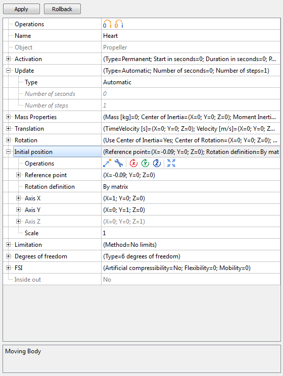
Body positioning:

It is extremely important to correctly position the moving body within the computational domain (parameter - Initial position). For some tasks this is critical and the entire joint calculation may suffer if the body is positioned incorrectly.

Resizing the moving body:

Another important point is the size of the moving body. If the Abaqus project is using a measurement system other than SI, then the moving body from Abaqus must be rescaled in FV by applying a scale factor in the properties of the moving body. Scaling should be performed like this, since this is the only method that ensures rescaling at each exchange step (not to be confused with Transformation).

Note! When applying a Transformation operation, you lose the connection with the original form of the geometric object. Therefore, for joint calculations, the initial position and scale should be adjusted only within the properties of the moving body.

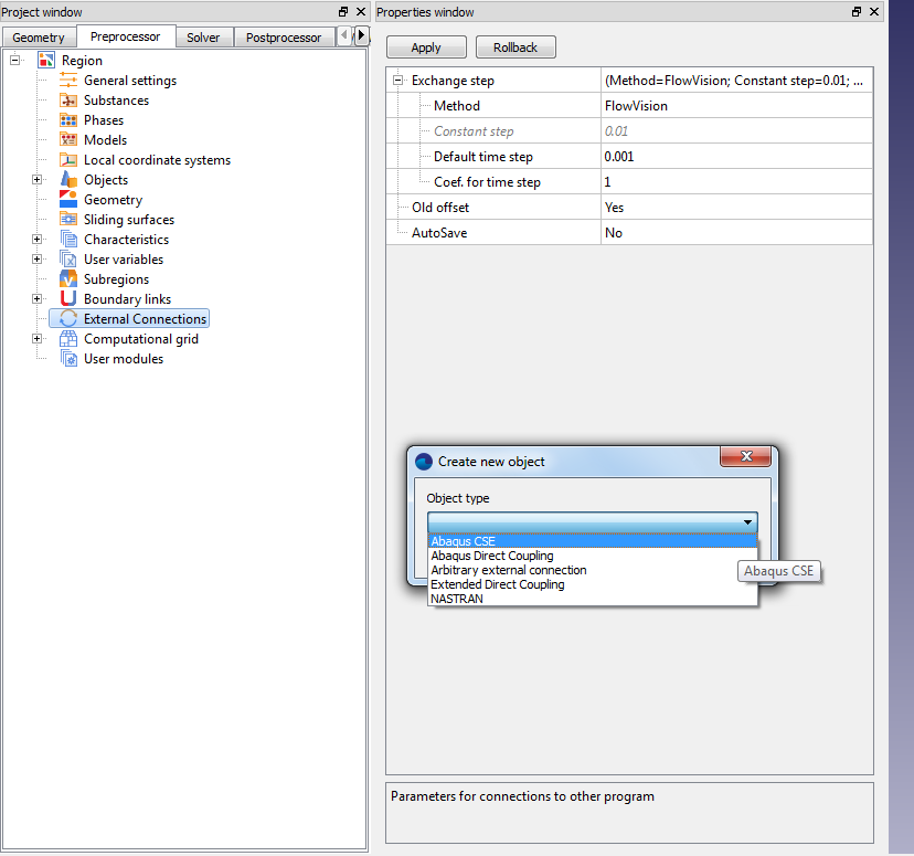
Creating a connector

As described in the 'Configuring the Abaqus project' section, an external connection with Abaqus is established using one of the two types of connectors : ‘Direct Coupling’ or ‘CSE-connector’.

To create a link, right-click on the External Links section in the project tree - "Create New Object", and select the required connector.

External communication settings

Among the connector settings, stress / heat relaxation should be noted. The first is used in models with deformation due to external loads, and the second is for problems with deformation due to temperature. For both types of relaxation, you can set:

• scale factor (loads will be scaled according to the specified value)
• start / end in steps (you can start transferring loads not from step zero, but later)
• initial / final coefficients (these reflect how the loads will be transferred - immediately and in their entirety or gradually with some gradient (ramping))

For example, you can set up the load transfer to happen smoothly over steps 1 to 50, by setting the following values:

There are similar settings for the transfer of heat loads.

These settings are needed to smoothly transfer the load from FV to ABQ, which will ensure a more stable solution at the beginning of the calculation. If these settings are not used, then your calculation may fall apart due to loads being applied instantaneously, which will result in large displacements of the finite element nodes in the FE-complex.

Running the FSI calculation

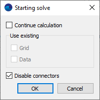
The first thing to do (and which should not be neglected) before starting any joint calculation is to make sure that the FV and ABQ projects can be simulated separately. To do this, you can run ABQ via CAE or from the command prompt (remember to comment out the co-simulation lines beforehand), and in FV turn on the "Disable connectors" option when starting the calculation (this option is not available if external links have not been configured).

If both projects run successfully and are calculated without errors, then you can proceed to running the FSI calculation. Typically, Abaqus is launched first, followed by FlowVision. During the calculation, it is important to monitor the results.

Running an Abaqus calculation

There are various ways to run Abaqus for FSI calculations, but the most common and convenient one is to run it from the command prompt. To do this successfully, you need to know the basics of scripting in Windows (or Linux - depending on which OS you are using) and also know the command words for Abaqus.

And so, in order to run Abaqus, you need to:

• be able to run a command line or write a batch script
• know the commands to navigate to the directory containing the Abaqus project
• know the parameters for running Abaqus for calculation together with FV

There can be any number of parameters in this line, tailored for each computer and its individual goals. A complete list of parameters can be found in the official Abaqus documentation. The article "Running joint calculations in FV and Abq" lists the minimum set of parameters that you need to know in order to run Abaqus with a CSE connector.

Running a FlowVision calculation

There are several ways to launch FlowVision, choose whichever is most convenient for you:

• via the PPP
• via the Terminal
• from the command prompt

After starting the calculation, make sure that the calculation is actually running. This can be done by looking in the Solver window - if the calculation has launched successfully, it will be performing calculations and the information it displays will be getting updated. Alternatively, you can check by connecting via the Viewer module and observing the simulation results (similarly, you can observe them in the PPP in the view window, however, body deformations will not be displayed there).

Monitoring results

You can monitor the solution both during and after the calculation process by using:

• layers (contour fills, graphs, etc.): in the PPP while connected to the Solver, in the Viewer module while connected to the Solver, in the Viewer module looking at saved layers (.fvvis files)
• characteristics (average values of variables): in the PPP, in the Viewer module, or by saving output to an Excel file
• graphs in the monitoring window: In the PPP or Viewer module while connected to the Solver

Note that displaying graphs in the monitoring window is a very useful feature that will help in monitoring a project while it’s solving and debugging it if necessary. To help control the simulation for ‘correctness’, make sure to plot graphs for:

• time step
• explicit time step
• maximum and minimum pressure in the domain
• maximum and minimum velocity in the domain
• other parameters that may be important to a specific task. For example, inlet mass flow rate.

With this data, you can track the behaviour of the project. Then, if the values become non-physical, you don’t need to wait for the program to crash out and terminate or for the calculation to complete, but instead stop it yourself and restart it, having corrected the input data / grid / time step. This will save a lot of time.

A description of how to plot the graph of a variable in the monitoring window can be found in the documentation.

Troubleshooting a project

One of the tools that can be used to troubleshoot a project are special debug visualization layers (cell set, cell debug). We have already talked about their capabilities in detail in the article ‘PostProcessing in FlowVision: Debug Layers’. We recommend checking  it out before you begin running projects. In short, if something goes wrong, debug layers can help you quickly identify problem areas in the calculation and look for the problem locally.

Since FSI projects are quite complex, almost each one will require some debugging. If you find yourself having difficulties troubleshooting a project yourself or if you have any questions, write to us at support@flowvisioncfd.com, and we will be happy to help you.