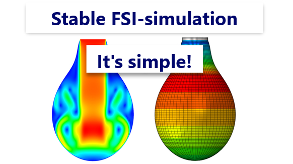
Our Team represents article about Stabilization methods of co-simulation on the example of filling air balloon with water.
The FSI model stability can be obtained by damping parameters (in third-party FE-code) and artificial compressibility coefficients (in FlowVision). In case of setting abnormally high values of artificial compressibility coefficients, the mass conservation is lost. In the same time, inflated damping coefficients may lead to non-physical behavior of the system. The methodology for the combined selection of these coefficients to achieve a stable calculation process with physical results is presented below.
Considering the process of filling an air balloon with an incompressible liquid, Abaqus will be used as a third-party FE-code. So, let's start with the creation of Abaqus project.
Abaqus project
The task will be solved in 3D.
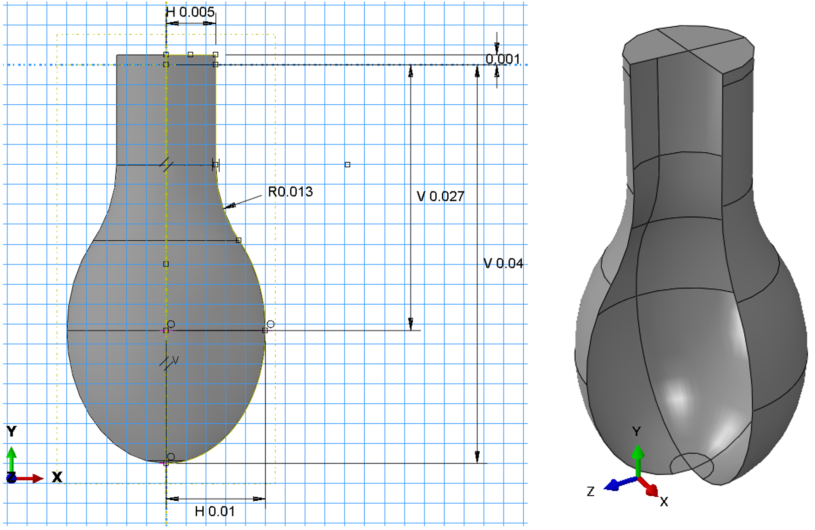
Geometry
The sketch of the balloon geometry consists of an ellipse, a rounding and a rectangle.
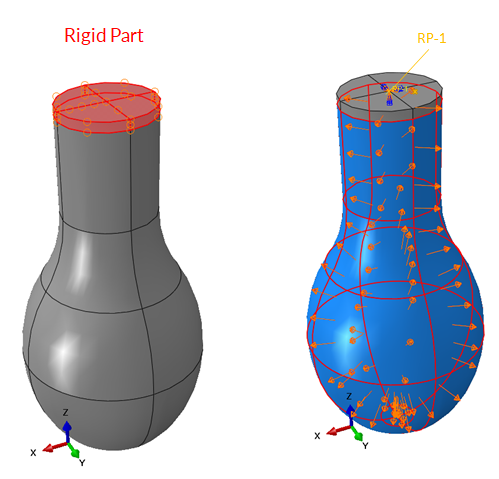
Boundary conditions & loads
The upper part of the balloon neck is modeled rigid and connected to the node by a reference point RP-1. In turn, this node is fixed by all degrees of freedom. Hydrostatic pressure is applied to the balloon.
Air Balloon Material Model
The Ogden hyperelastic material model of the fourth degree is used as a model of the air balloon material. Models of hyperelastic materials are determined by the specific potential energy of elastic deformation, in our case:
![]()
where α1 = 1; α2 = 1.3; α3 = 5; α4 = –2; μ1 = 0; μ2 = 4.1e5; μ3 = 3e3; μ4 = 10e4; D1 = 9.47e –11; D2 = 0; D3 = 0; D4 = 0.
FlowVision project
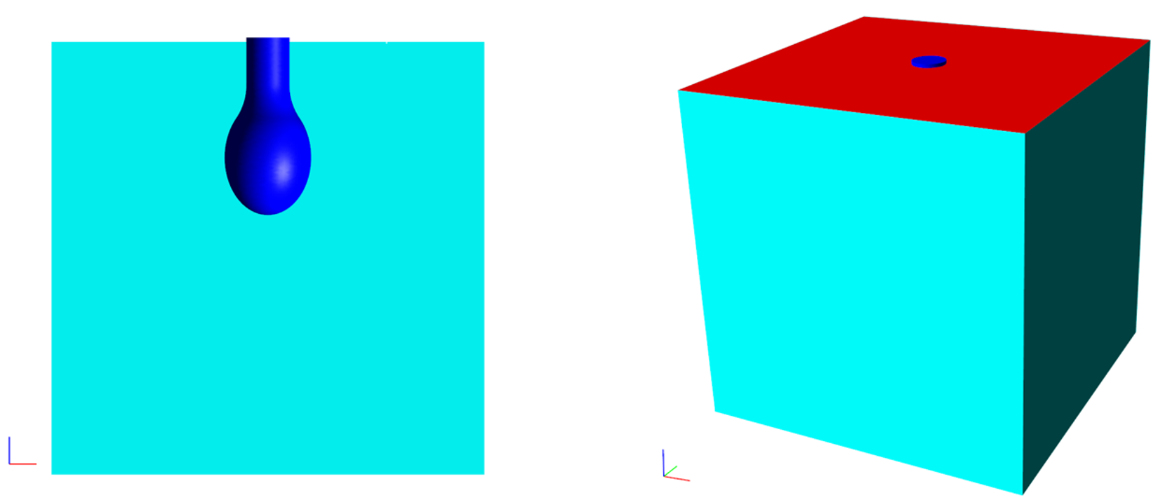
Geometry
Geometry of the balloon has to be placed into the computational domain (for example, cube). Size of the cube should be large enough to fit the air balloon in its maximum volumetric state. Rigid part of the neck should be outside the cube as a noncomputed (rigid) object. Since it is assumed that the computation space will be inside the ball, the imported object should be "turned inside out".
To set a Substance
Liquid state of uncompressible water with constant density and dynamic viscosity will be taken as a working fluid:
![]()
Fluid motion is defined by the Navier-Stokes equations.
Boundary conditions
Boundary condition Wall with no slip condition is set to the surface of the ball and the side + bottom faces of the cube. Inlet/Outlet with constant velocity boundary condition is set to the top surface of the cube, what corresponds to filling with tap water.
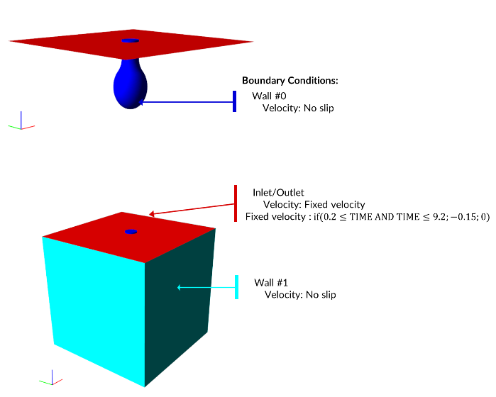
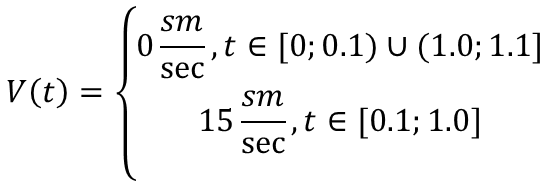
Let's consider water starts filling balloon at time t = 0.2s and is poured for 9 seconds at velocity of 15 cm/sec.
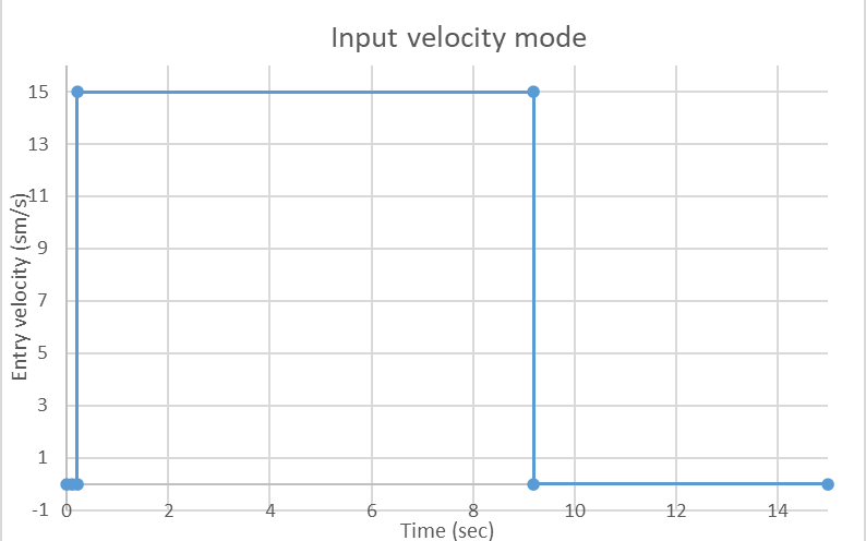
The shown input speed mode can be easily described by the following logical expression, by using integrated Formula editor (but please, don't forget to convert cm/s to m/s):
![]()
About the stability of the FSI-model
Artificial compressibility coefficients (FV)
To stabilize a co-simulation, the following coefficients are used from the FlowVision side:
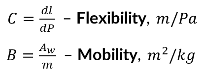
dl – displacement of the body's surface at the pressure increment at the given time step dp;
Aw – area of the body's surface that interact with the fluid;
m – the body's mass.
The formulas presented are initial estimation, so variation is required.
The following estimations can be given for the artificial compressibility coefficients:
- Lower limit: stability of FSI-simulation
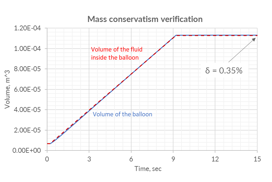
- Upper limit: the mass conservation
The volume of fluid inside balloon after water filling is one of the defining parameter. With higher than normal coefficients of artificial compressibility, the volume of water inside the ball may be less than the volume of water flowing in, which is obviously not physical.
Damping coefficients (ABQ)
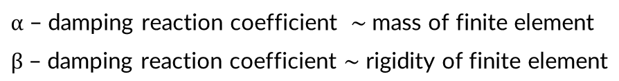
Oscillation frequencies of the structure could be limited by using those coefficients, thereby pressures near the walls will be calculated more accurately.
The following estimations can be given for the coefficients of damping reaction:
- Lower limit: stability of FSI-simulation
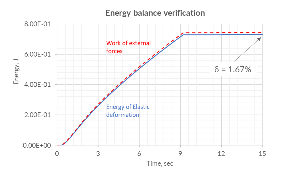
- Upper limit: approximate implementation of energy equation: Wext = Uel
Wext – work of external forces, J
Uel – potential energy of elastic deformation, J
Defining the coefficients
Artificial compressibility coefficients
Let's set damping coefficients α = 1e5; β = 0.1 in the ABQ project for initial approximation.
To define flexibility one have to start next calculation using Abaqus (not FSI): an internal uniform linearly increasing pressure is applied to the ball. The movement of the node in the pole has is determined.
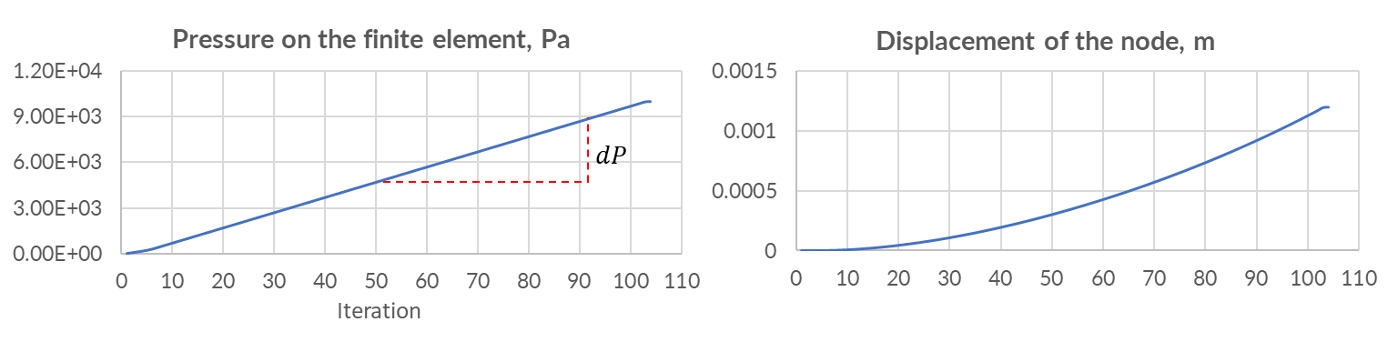
Ratio of displacement increment to pressure increment - this is the flexibility coefficient.
![]()
To define the coefficient of mobility one has to know the surface area of the deformable part of the air balloon (can be extracted from FV) and mass of the body (can be extracted from ABQ):
![]()
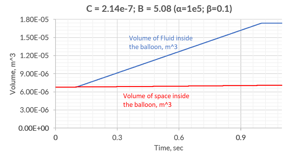
As for now, we have coefficients of artificial compressibility for initial approximation. Let's start trial FSI-simulation with artificial compressibility coefficients and damping coefficients for the following input velocity mode:
With a zero-order approximation of the coefficients, the conservativism of the mass is not preserved:
In case of reduction of artificial compressibility coefficients, one can achieve error within 6%:
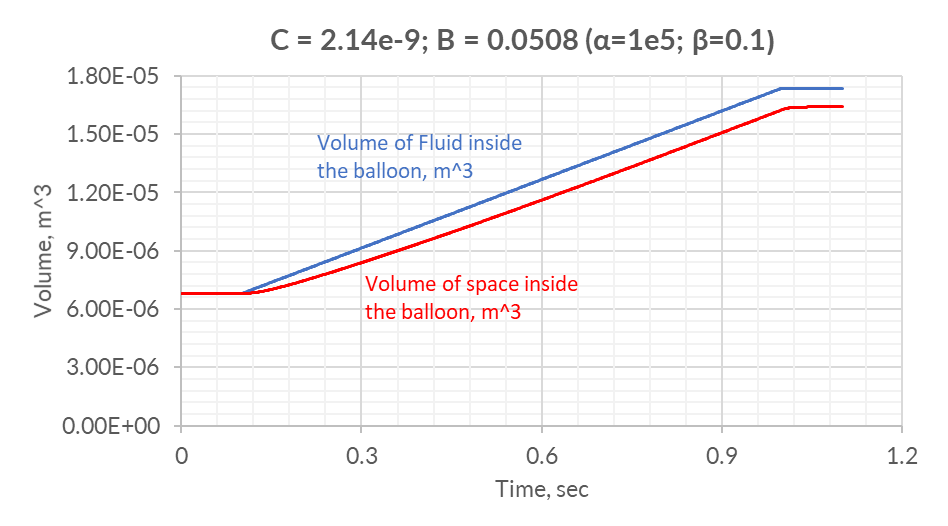
Values of C = 2.14e-9; B = 0.0508 will be chosen as initial, then we will reduce the values of damping coefficients.
Damping coefficients
It is necessary to obtain damping coefficients at which the work of external forces Wext and the potential energy of elastic deformation Uel differ slightly, i.e. the relative error:
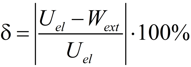
should be as small as possible.
After carrying out some number of FSI-simulations the following damping coefficients are chosen: α = 1e5; β = 0.025 (C = 2.14e-9; B = 0.0508).
Results
The selected values of the coefficients of artificial compressibility allowed us to obtain a stable calculation in which:
- the highest relative error of potential energy and the work of external forces was 1.67%.
- at the end of the simulation, 0.35% of water mass was lost.
Put it in a nut shell
To get a stable FSI-simulation, one has to often damp the system and (or) add artificial compressibility coefficients. To get a stable calculation with physical results, it is necessary to choose the optimal combination of stabilizing coefficients. Using the algorithm shown in the example with filling the air balloon can reduce the time for selecting these coefficients.
If you have any other questions left, please feel free to write us support@flowvisioncfd.com