This functionality provides many opportunities for increasing accuracy of calculations while using less computational resources.
For your tasks, you can use:
- volume / surface adaptation;
- adaptation for curvature / sharp edges;
- adaptation by condition / to solution;
- merging.
Types of adaptations
All adaptations in FV can be permanent or periodic, and can be activated by time or step. Depending on the problem being solved, different types of adaptation can be used to improve calculation efficiency.
- Adaptation by surface / in volume
- Adaptation for curvature
- Adaptation for sharp edges
- Merging
- Adaptation to solution
- Adapration by condition
Adaptation by surface / in volume
Used for local refinement of the computational mesh along the surface / within the volume of a geometric object. An object for adaptation may be:
- standard geometric FlowVision object: plane, box, cone / cylinder, ellipsoid / sphere;
- imported object;
- supergroup;
- boundary condition.
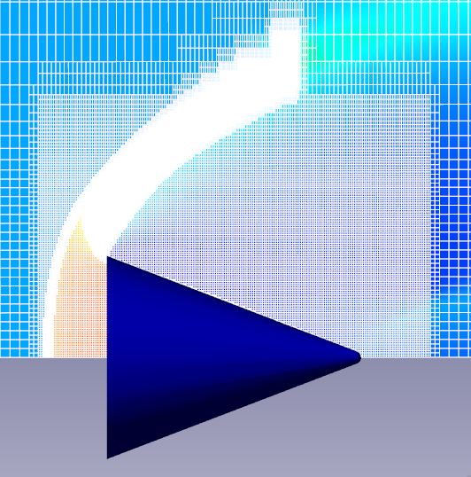
In the example of modeling the Kármán vortex street with flow around a cube, an adaptation in the box volume (1) refines the resolution in the vortex flow region, and an adaptation along the cube surface (2) - in the boundary layer region. This is necessary to more accurately determine the forces on the surface, as well as the flow parameters in the region of the disturbed flow.
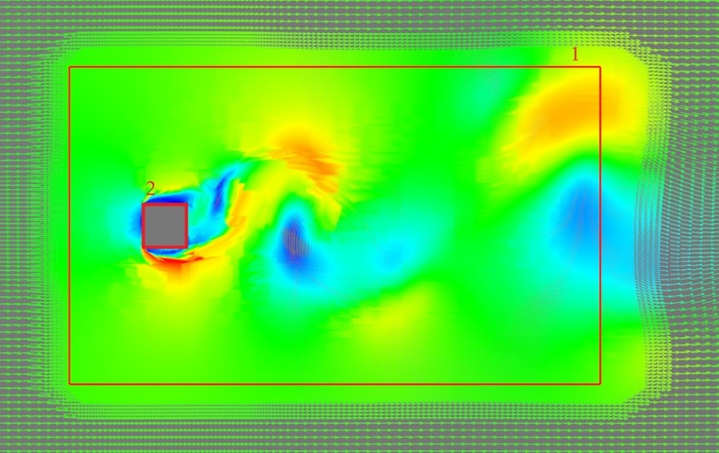
Velocity field distribution in a computational grid with adaptations in the volume (1) and on a surface (2) when modeling the Kármán vortex street
properties window
The adaptation properties are determined by the parameters: Max. level N - the level of subdivision of the cells in the computational grid and the number of layers for level N - the number of cells in one level of subdivision.
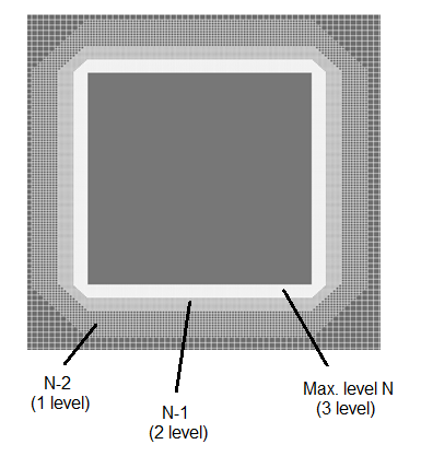
For volumetric objects layers are built outwards, for surface objects - to both sides of the surface.
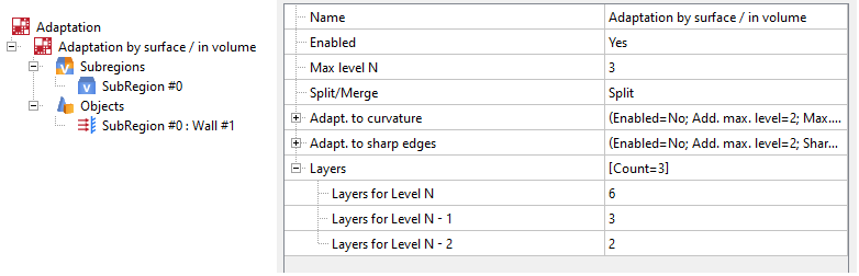 Adaptation properties window for geometric objects
adaptation for curvature / sharp edges
Used for local refinement of flow parameters near complex geometry. Adaptation for curvature or sharp edges may be turned on in the properties window for Adaptation for geometric objects.
Use surfaces (supergroups or boundary conditions) as objects for adaptation.
The adaptation for curvature / sharp edges is not active for volumetric objects
Adaptation for curvature
Used to adapt curved surfaces. For example, to determine the flow parameters near the point of complete deceleration of flow around an airfoil.
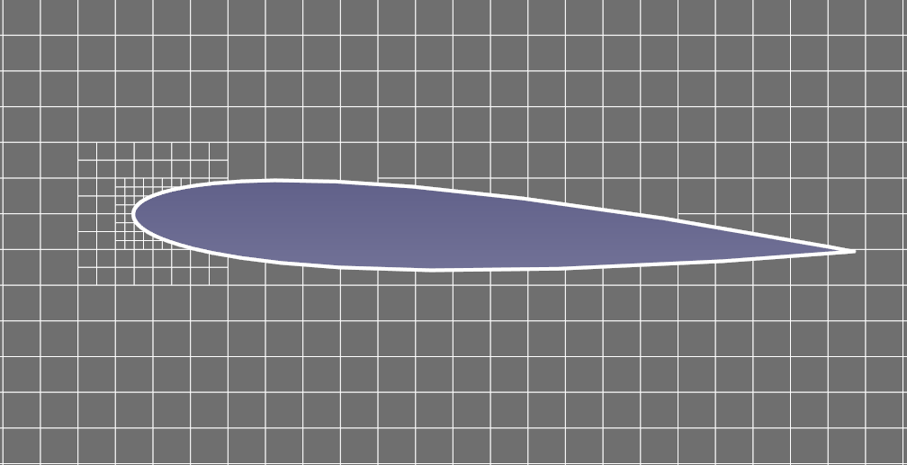 The second level of adaptation on the curved surface at the nose of the NACA 012 profile
Properties window for adaptation for curvature
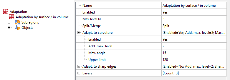
Add. Max. level - number of additional levels to the maximum adaptation level set by Max. level N. Put simply, this number of levels will be added to the maximum level N.
Max. angle - the maximum value of the angle between the inner normals of the facets at which the curvature adaptation is triggered. The more curvature a surface has and the rougher the presented geometry is, the higher the angle value should be set.
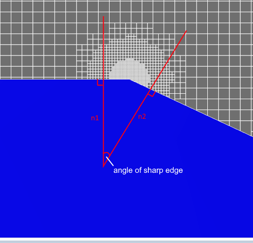
adaptation for sharp edges
Used for local refinement of flow parameters near sharp edges of geometric objects. For example, you can resolve areas with maximum stresses - the edges of gears when simulating flow inside a rotary compressor.
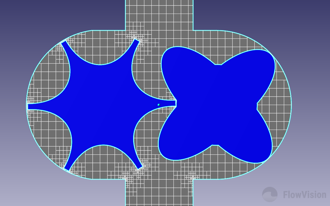 4 level adaptation on sharp edges of compressor gear
Properties window for adaptation for sharp edges
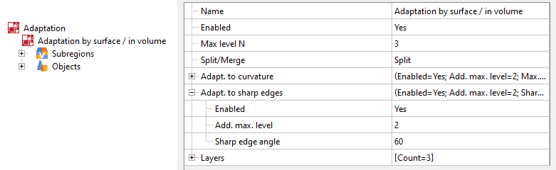
Add. max. level - number of additional levels to the maximum adaptation level set by Max. level N.
Sharp edge angle - the maximum value of the angle between the inner normals of adjacent facets, at which adaptation on sharp edges is triggered.
The number of layers only needs to be set for basic adaptation of levels N, N-1, etc. For those additional adaptation levels specified for curvature / sharp edge adaptation (for N + 1, N + 2, etc.), the number of layers is assumed to be equal to the maximum adaptation level (N) and is applied to all levels above.
For the maximum level of common adaptation (Max. level N) and for the level of adaptation for curvature / sharp edges (Max. level N + Add. max. level), the number of layers is the same
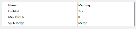
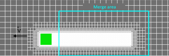
Merging
Merging acts inversely to the adaptation of splitting - it eliminates the excessive refinement of cells in the computational grid. If you select Adaptation Split / Merge = Merge in the properties window, all cells with a split level greater than the one specified in Max. level N will be removed. After merging, the maximum adaptation level will be equal to Max. level N.
Cases when it is recommended to "merge" excess adaptation:
- when setting motion for an adaptable body - to get rid of the adapted trace behind the moving body;
- using adaptation by condition - the solution can change over time / simulation and, therefore, in some areas of the grid, adaptation loses its relevance;
- if you mistakenly (or intentionally) set many levels of adaptation at once.
adaptation to solution/ by condition
These adaptations are useful in cases when it is not known in advance in which area of the computational space it is necessary to refine the computational grid. The place of splitting will be found in the process of simulation, depending on the values of the calculated variables, which allows to save computational resources as much as possible.
Adaptation by condition is useful when you need to more accurately resolve a region within a specified range of variable values. Adaptation to solution refines the computational grid around cells in which either the value of a computed variable is close to a specified one, or where a sharp gradient for this variable is observed.
These types of adaptation are similar and interchangeable. Consider the effects of its application when choosing an adaptation.
Let's consider the aspects of applying adaptations by condition and to solution in the example of supersonic air flow around a cone with shockwave formation. Initially, the calculation uses a grid consisting of 23,000 cells, with adaptation inside a box. An estimated distribution of the flux density was obtained using such a grid.
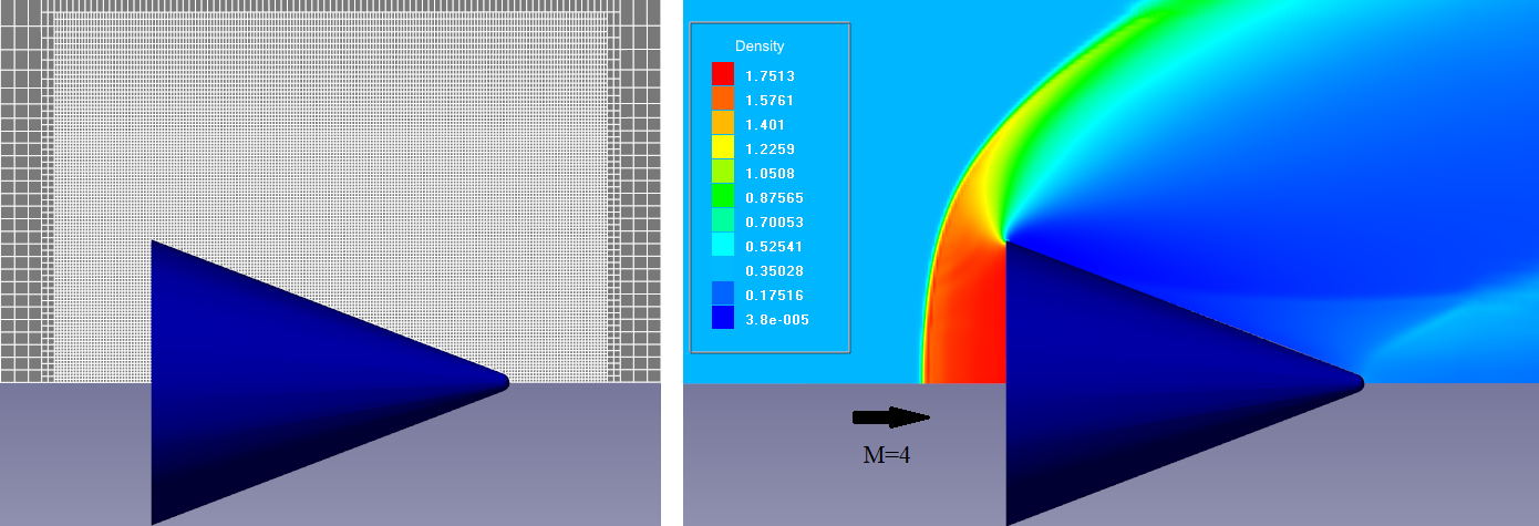 Computational grid and density distribution for external supersonic flow around a cone
To resolve the shockwave parameters, you can adapt the mesh in the box (see figure above). However, it is not known in advance where the shockwave will appear - the adaptation area will be vast. To reduce the number of over-adapted cells, we use adaptations to solution or by condition. Let's continue to adapt the mesh!
adaptation to solution
Adaptation to solution allows to refine the computational grid around cells in which either the value of a computed variable is close to a specified one, or where a sharp gradient for this variable is observed. To apply the adaptation, it is necessary to indicate the maximum adaptation level (Max. level N), select a variable, then set its value or select the gradient of this variable. It is also necessary to specify the total number of computation cells, upon reaching which the adaptation to solution will stop refinement.
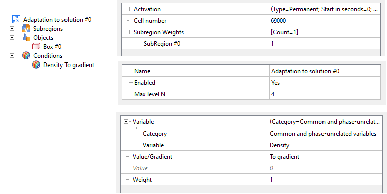
Properties window for adaptation to solution (to gradient)
Some FEATURES OF APPLICATION
- Adaptation to gradient may be applied from the beginning of the calculation.
In this case, the computational grid will be adapted starting from the 1st iteration. This feature allows to avoid using preliminary calculation to estimate a variable range (used to apply adaptation to a specified value) for faster calculation.
- Adaptation is dynamic and does not require merging.
There is no need to set merging of over-adapted cells. The adaptation independently changes its position on the computational grid, depending on the value of the calculated variable.
- There is a limit on the number of cells that may be adapted.
Thus, it is possible to limit the task dimension in advance. Refinement will continue until the number of cells in the computational grid exceeds the threshold value in the limiter.
The "Number of cells" parameter includes all cells in the Subregion: calculated and non-calculated (cut from the Subregion by a moving body)
- It is not allowed to specify the number of layers for each level of adaptation.
Since the adapted cells are those with a specific value of a variable, this limitation does not allow to create smooth adaptation in the area (see picture below - "spots" and "pieces" of adaptation are observed). The existence of sharp transitions between regions with different adaptations reduces solution accuracy.
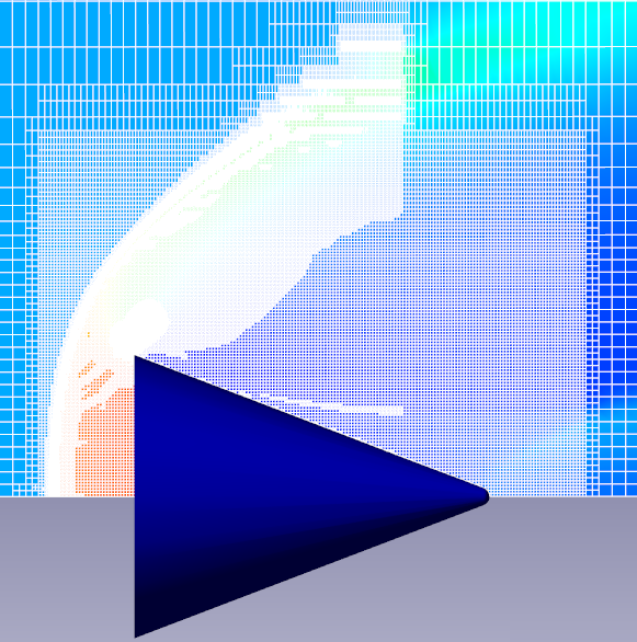 Shockwave resolution by adaptation to solution: computational grid (68,221 cells) and density distribution
adaptation by condition
Adaptation by condition can be used if you need to more accurately resolve a region within a specified range of variable values. To apply this type of adaptation, it is enough to select the Variable and indicate the range in which the specified level will be adapted to these values (Max. level N).
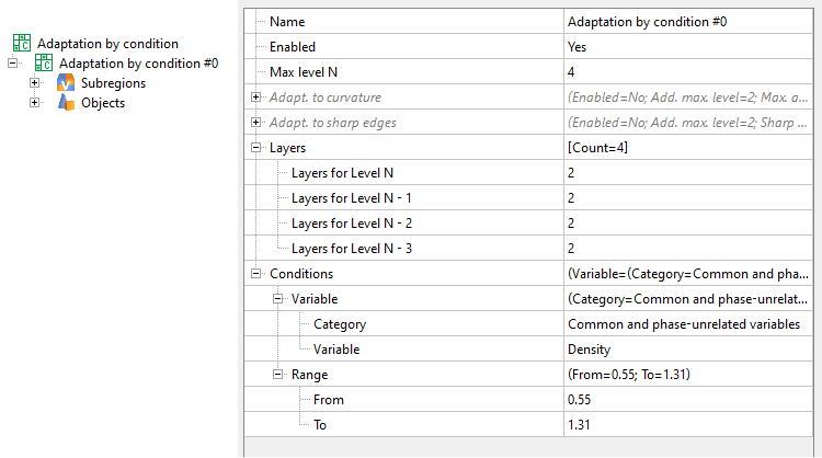 Properties window for adaptation by condition
Some FEATURES OF APPLICATION
- Specifying the number of layers for the maximum and intermediate adaptation levels allows to create a smooth computational grid which, of course, affects the solution accuracy.
 Shockwave resolution by adaptation by condition: computational grid (68 830 cells) and density distribution
Otherwise, the computational grid can adapt without ever stopping, especially over a wide range of values for a given variable.
- Adaptation by condition, as a whole, completely replaces adaptation to solution.
RECOMMENDATIONS ON how to USE ADAPTATION TO SOLUTION / by CONDITION:
To obtain a computational grid with adaptation to the value of a computed variable, it is necessary to carry out a preliminary calculation - to determine the variation range of a value. Based on the obtained data, for the main calculation, it is then required to indicate this value range, specifying:
-
- maximum/minimum values for the entire range. (The result is similar to the one obtained using the adaptation to solution, to gradient).
- a specific value for the computed variable. (Similar to adaptation to solution, to value).
- Adaptation by condition requires more computational resources and time.
The absence of restrictions on the number of cells, as well as the need for pre-calculation, leads to a significant decrease in the calculation speed.
useful hacks for adaptations
The use of adaptation goes hand in hand with the study of grid convergence: determining for which combination of different adaptations the solution does not depend on further refinement of the computational grid.
Below we will discuss three techniques for using adaptations:
- Setting a constant width of adaptation zone - reduces the number of calculation cells.
- Grid Convergence Automation - FV will perform grid convergence investigation calculations while you may have a rest.
- Periodic activation of adaptations - just saves you time.
Setting a constant width of adaptation zone
The adaptation zone width is determined by a set of adaptation layers - a set of cells at the same refinement level.
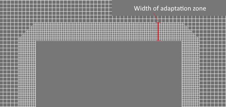
It's good to remember that the width of the adaptation zone can change when you are specifying a sequential surface adaptation (Fig. Case 1). It is necessary for the width of the adaptable layer to be unchanged during the calculation if you want to resolve by grid only a studied area with maximum flow disturbances (Fig. Case 2). This requires changing the number of layers for each new level in the adaptation properties.
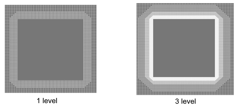 Case 1. If the number of layers remains unchanged
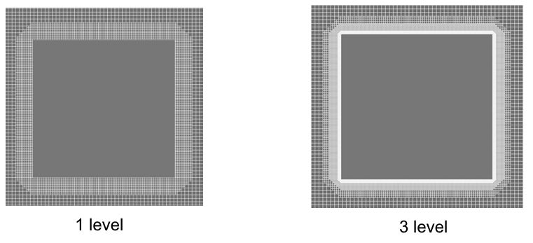 Case 2. The number of layers is changed to maintain the thickness of the adaptation layer
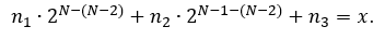
Since the next level of adaptation splits the cell of the current level into two in each direction, it is convenient to use the following formula to calculate the number of layers for each level of adaptation, depending on its level. Let there be x layers at the initial adaptation level N-2. For the adaptation of level N, we'll define n1, n2, n3
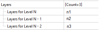
from the equation:
Grid Convergence Automation
To automate the process of grid convergence investigation, it is convenient to apply adaptation using the formula or table that depends on time or step number.
With adaptation (that is, with a decrease in the size of computational grid) the time step decreases. This means that the time intervals between steps will become uneven.
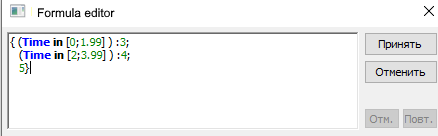
how to set adaptation by formula editor
An example of setting adaptation of 3-5 levels, depending on the current time, on the surface of the Boundary condition "Wall":
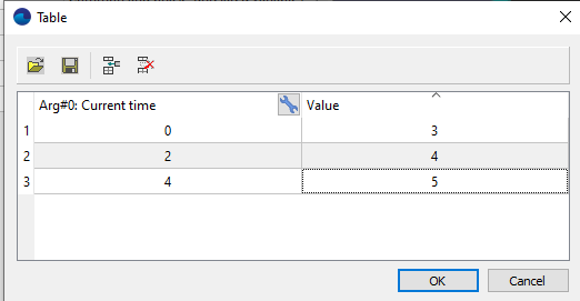
how to set adaptation by a table
An example of setting adaptation of 3-5 levels, depending on the current time, on the surface of the Boundary condition "Wall":
RESULTs OF AUTOMATION OF THE PROCESS OF DETERMINING THE grid CONVERGENCE
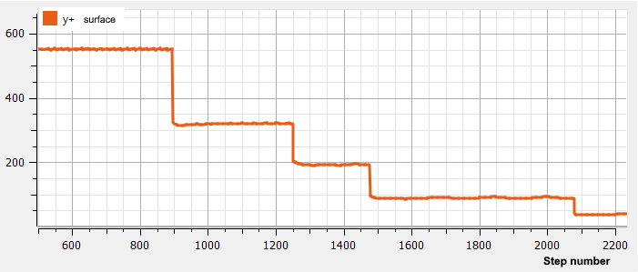
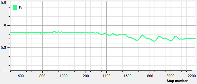
Investigation of grid convergence: at Y+ = 44, the value of the longitudinal force is constant
Periodic activation of adaptations
(by time or by step)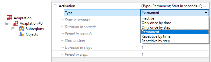
The main advantage of using periodic adaptation is a significant decrease in calculation time. Periodic activation of adaptation does not impair the accuracy of calculation, but simply allows you to perform the adaptation process of the calculation cells less often: even setting the periodicity at only 20 steps will significantly speed up your calculation.
The use of a periodic type of activity is effective:
- for periodic application of adaptation to the solution in order to save computational time.
- when adapting the surface of moving bodies. Set merging for adaptation in the area behind the body to be performed periodically, and not at every iteration.