This article will be useful for the beginners who want to learn more about the turbulent flow and pitfalls encountered during its modeling. We'll go through:
introduction
Let's start with the Breadshow definition of turbulence:
Turbulence is a three-dimensional unsteady motion in which, due to the extension of the vortices, a continuous distribution of chaotic pulsations of the flow parameters (velocity, pressure, etc.) is created in the range of wavelengths from the minimum determined by viscous forces to the maximum determined by the flow boundary conditions.
In other words turbulent flow is a flow in which motion is random in time and space.
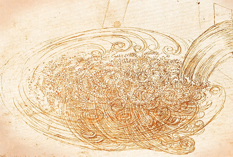 The turbulent flow by Leonardo da Vinci
The laminar flow, in contrast to the turbulent one, is structured. The medium in this flow moves by layers, without mixing and pulsations. The figure below shows the laminar-turbulent transition in the flow: the processes of intensive mixing and vortex formation occur during the transition.
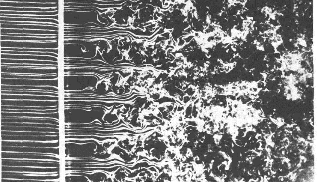
Changing the flow from laminar to turbulent
LAMINAR AND TURBULENT FLOW velocity PROFILES
Let's consider the flow in a pipe of circular cross section and infinite length.
Jean Louis Poiseuille determined that the laminar flow has a parabolic velocity profile. The velocity profile changes to some other form during the transition to a turbulent flow. Changes in the velocity profile are caused by inertial forces acting on particles in the flow. In other words, the profile of the averaged velocity of the turbulent flow in pipes or channels is characterized by a rapid velocity increase near the walls and less curvature in the central part of the flow.
Laminar flow in tube Turbulent flow in tube
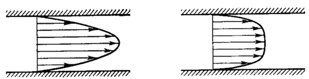
Velocity profiles for laminar and turbulent flow
For a turbulent flow velocity is described by a logarithmic law (that is, the velocity linearly depends on the logarithm of the distance to the wall) except a thin layer near the wall.
Reynolds number
Usually, when somebody speaks about a turbulent flow, one immediately recalls the Reynolds number (Re). In fact, it is the ratio of inertial forces to viscous friction forces.
![]()
Here ρ - density, V - velocity, l - characteristic geometric size, μ - dynamic viscosity of the medium (table value).
For a flow characterized by a low Reynolds number, the stream will mainly depend on the viscous forces. At high Reynolds numbers, the influence of inertial forces prevails, and as a result turbulences arise.
To determine the boundary between the laminar and turbulent flows, the concept of the critical Reynolds number is introduced (Recr):
- Characteristic Re < Recr – laminar flow
- Characteristic Re > Recr – turbulent flow
The critical value of the Reynolds number for different medium will differ:
- water: Recr ~ 2200
- air: Recr ~ 105
Where do the turbulent flows appear in the real life
As it was noted earlier, the turbulent flow differs from the laminar flow not only by the velocity profile, but also by the presence of intense vortex formation. Therefore, the phenomenon of turbulence significantly affects the calculation results and must be taken into account.
The fields of application for turbulence are endless: aircraft, automotive industry, shipbuilding - modeling air motion around airplanes/cars/ships, ventilation and air conditioning - modeling air flows in rooms, ventilation shafts, aircraft and automobile cabins; a separate vast area is represented by biomechanics - blood flow modeling in the chambers of the heart, around heart valves, etc.
turbulence modeling
There are three main approaches for mathematical description of the turbulent flow:
- Direct Numerical Simulation (DNS);
Turbulent flows are simalated by solving the Navier-Stokes equations directly. The three-dimensional non-stationary equations are used for modeling regardless to the flow nature. This approach requires a sufficiently accurate resolution of the computational grid in all areas where vortex formation occurs, therefore its application is limited by the performance of computer technology. The grid step in this case should be of the Kolmogorov scale.
The concept of Kolmogorov scale
According to the Kolmogorov hypothesis, the lower bound on the magnitude of the structures involved in the process of energy dissipation may be estimated.
The scale ηĸ, that is called Kolmogorov, characterizes the linear dimensions of structures, on which viscosity still has a significant effect.
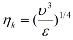 , where ν -kinematic viscosity, ε - energy dissipation.
- Large Eddy Simulation (LES);
This approach is between the DNS and RANS approaches. The filtering of turbulent flow characteristics from short-wavelength inhomogeneities is used in it. That is, the averaged Navier-Stokes equations are solved (as in RANS), but averaging is made over regions with sizes of the filter. A system of averaged Navier-Stokes equations is formed after the filtering procedure. This system is applicable to regions larger than the filter. The averaged equations are closed using the “subgrid” turbulence model. The vortex structures with dimensions exceeding the dimensions of the filter (computational grid) are resolved accurately, and smaller vortex structures are modeled.
- Reynolds Averaged Navier-Stokes (RANS) – approaches based on averaging the Navier-Stokes equations over the Reynolds number. To take into account the energy loss due to vortices that are not resolved by the computational grid, the concept of averaged velocity is introduced (this is described in details below). A new unknown - the Reynolds stress - arises during the equations averaging. So it becomes impossible to solve the Navier-Stokes equation with the continuity equation. Therefore, turbulence models are additionally introduced to close the system of equations (for determining the Reynolds stress).
Turbulence model is a mathematical model that allows to describe the flow behavior with the desired accuracy. As applied to RANS approaches, the turbulence model is a set of additional equations designed to close the Navier-Stokes system of equations after it has been averaged over Reynolds.
The turbulence models differ in the constants that are set in these models, as well as in the turbulent viscosity determination. The constants are predominantly empirical, and they are selected according to the characteristics of the particular task. Turbulence models can include from one to several equations, and the more equations there are, the more computing resources are required.
RANS approach allows to obtain only an averaged flow and describe it if there are pulsations in the velocity around a certain average value. This approach allows to get good results on a coarse mesh. The LES approach allows to resolve vortices that affect the nature of the flow. The results of this analysis will be more accurate, however, a larger number of calculation cells and a smaller time step will be required. To resolve all the vortices and pulsations, it is necessary to solve the equations directly (DNS): to create a fine mesh, the cell size of which will allow to resolve one vortex by several cells. The time step, respectively, should be such a value that the vortex rotation period will be also time-resolved by several steps. This approach is extremely resource-intensive and is rarely used in engineering calculations.
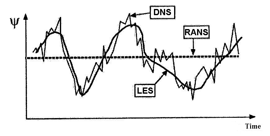
The difference in approaches on the example of the flow velocity
The main concepts
ENERGY DISSIPATION
The energy transfer in a turbulent flow occurs in a cascade manner: energy comes from the averaged flow to the largest vortices and is subsequently transferred to more and more small vortex structures. As a result, it reaches ultrasmall vortices (with Kolmogorov scales). They dissipate kinetic energy and transfer it to a thermal state.
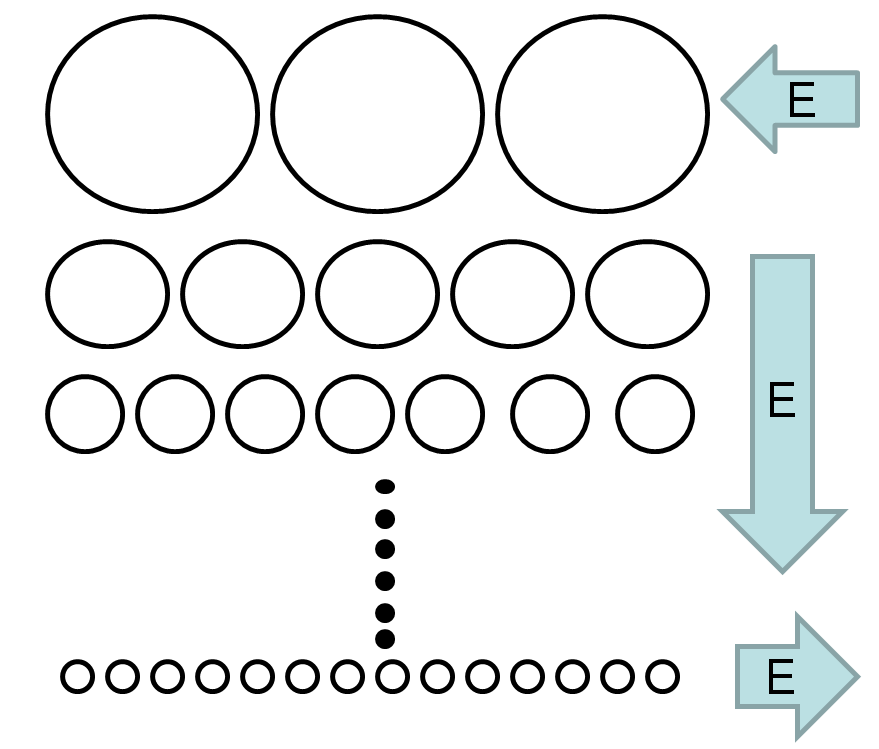
Cascade energy transfer in a flow
Pulsations
The transition from laminar to turbulent flow is characterized by vortex formation. The result of the chaotic motion of particles participating in turbulent mixing is the pulsation of their velocity. Therefore, in RANS approach the velocity projections can be divided into the average component and the pulsation additive:
![]()
The pulsating motion of particles, in its turn, is a source of pressure, temperature and density pulsations. The degree of flow turbulence is a measure of pulsation intensity.
The momentum transfer through the vortices is taken into account due to the additional turbulent viscosity. If we substitute the expressions for the averaged velocities into the Navier-Stokes equation and transform them, in the end some terms will be reset to zero, but the product of the averages and the product of the pulsating components will remain. The product of the pulsating components - a new unknown - is called the Reynolds stress. With this new unknown it is impossible to solve the Navier-Stokes equation together with the continuity equation. Therefore, the system of equations must be closed.
For this, the Businesk hypothesis was introduced: to consider the Reynolds stress approximately the same as the friction stresses that are associated with viscosity, i.e. like a certain viscosity, multiplied by the flow deformation. Therefore, a new variable appears - turbulent viscosity, which makes it possible to take into account the additional integral effect of the vortices, although they are not resolved by the grid.
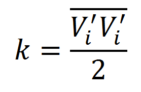
TURBULENCE KINETIC ENERGY
The concept of kinetic energy of turbulence (k) was introduced by Prandtl. It is, in fact, the specific kinetic energy of vortices in a turbulent flow or the root-mean-square velocity pulsation.
Prandtl noted that the pulsation along y axis in the flow, which consists of the turbulent layers with vortices, is the same as along the x axis. A vortex can change its gradient in velocity and is proportional to the turbulence scale. It was proposed to consider the path length of the vortex mixing as a turbulence scale.
Interaction of FLOW and WALL - what is Y+
The flow near the wall looks like a laminar one - everything moves in layers, then vortices appear, their number increases and the turbulent flow is already observed in the flow core.
Considering the coordinate of the distance from the wall in the coordinates (x, y), one can see various regions of the boundary layer. There are:
- viscous sublayer, where absolutely laminar flow is observed.
- the buffer layer - the mixing zone, where the Reynolds number begins to influence the flow and a turbulence appears.
- turbulent core (inertial layer and upper boundary layer) - the development of a turbulent layer, where the viscosity forces and the influence of the wall are already insignificant.
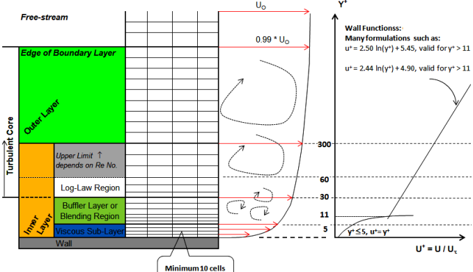
The layers scheme in the boundary layer
Considering the velocity profile in dimensionless coordinates, one can determine a number of quantities that describe the flow in the boundary layer:
- dimensionless velocity, which is equal to the ratio of the local velocity to dynamic velocity, determined only by shear stress on the wall.
dimensionless velocity:  dynamic velocity:
- dimensionless coordinate Y+ - distance to the wall reduced to dimensionless value due to the velocity of dynamic friction. The parameter Y+ can be considered as the local Reynolds number in the cell.
dimensionless distance to the wall:![]()
If the center of the first cell is located in the zone where Y+< 5, then it is a viscous sublayer and the flow is laminar — the profile is a parabola and also there is a parabola in the logarithmic coordinates. If 5 < Y+ < 15 then it is the mixing zone - in this place you need to connect two profiles: one is laminar, the second is turbulent. If Y+ > 30, then this is a zone of turbulence - and there is a straing line in thelogarithmic law. Depending on the region in which the center of the first cell is located, the appropriate approaches to modeling this region should be applied.
Two approaches to the modelling
high-reynolds approach
It is characterized by the fact that the wall region is poorly resolved by the grid and the center of the first cell does not fall into either the viscous or buffer sublayer (Y+ > 5). In this case, a relatively coarse mesh is constructed and nobody knows what happens in the boundary layer region. Then the near-wall functions are used for the near-wall flow calculation .
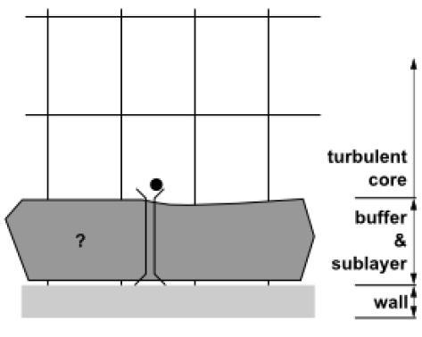
Coarse computation grid. The dot shows the center of the first cell
Wall functions are some empirical and semi-empirical dependencies designed to determine the velocity profile in the wal region.
FlowVision implements 2 models of wall functions: WFFV (Wall Function FlowVision) and WFS (Wall Function Standard). Read more about wall functions here.
Low-reynolds approach
It is realized if the center of the first cell lies inside the boundary layer. In this case, the wall region has a good mesh (Y + <1), the center of the first cell is obviously in the laminar zone. So, there is no reason to use near-wall functions, because in the center of each cell the velocity profile is constructed by the numerical solution.
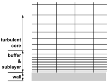
The flow with a fine mesh near the wall
turbulence modelling in FlowVision
turbulence models in FlowVision
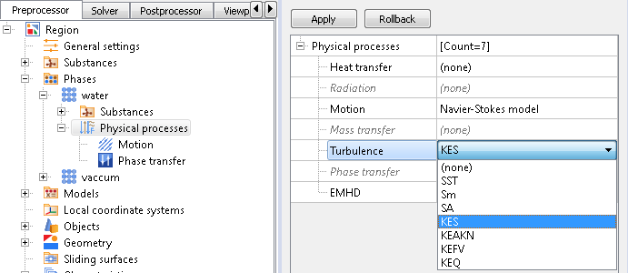
FlowVision implements 7 different turbulence models. You may use one of them depending on your task:
- KES (k-ε) – standard turbulence model. Its application is possible only in high Reynolds calculations (on a relatively coarse grid with wall functions)
- KEAKN (Abe, Kondoh, Nagano) – low-Reynolds model, which is recommended for use in low-Reynolds calculations (on a grid allowing a viscous sublayer near the wall, without wall functions).
- KEFV – k-ε model upgraded by FlowVision developers. The KEFV model may be used in both low-Reynolds and high-Reynolds calculations. In the first case, the laminar sublayer is meshed (wall functions are not used), in the second case, the laminar sublayer is not meshed (wall functions are used). This model satisfactorily predicts the position of the laminar-turbulent transition on a solid surface. In low-Reynolds calculations, it is necessary to specify the oncoming flow turbulence.
- KEQ (quadratic model) - the most full, but also the most "capricious" of all models. It considers a special element - the element of the vorticity tensor. This model is used for especially swirling turbulent flows, flows behind a back step and may only be used in high-Reynolds calculations.
- SST (Menter model) - is known for combining both the k-ε model and the k-ω model, which was developed for approaches to resolving the wall region. In this model, a new value - ω - specific dissipation of vortices - appears. The equations of the k-ω model are solved for this model in the wall region, and the equations of the k-ε model are solved in the region far from the wall.
- SA (Spalart-Allmares model) - one-parameter model that has been developed for aerospace applications. It gives good results for boundary layers characterized by positive pressure gradients. It can be used both in low-Reynolds and high-Reynolds calculations. Traditionally, this model works effectively in the low Reynolds case.
- Sm (Smagorinsky model) - algebraic model that does not require solving convective-diffusion equations. Sm model can be used only in low Reynolds calculations on a fine mesh.
how to set TURBULENCE IN FLOWVISION
It is necessary to set the physical process of Turbulence in the Phases tab by selecting one of the proposed turbulence models.
Turbulence models in physical processes
Turblence is set as pulsations and turbulent scale ( Prepocessor -> Models -> Initial data). These parameters determine the degree of the flow turbulization.
Pulsations: Turbulence scale:
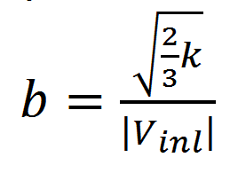
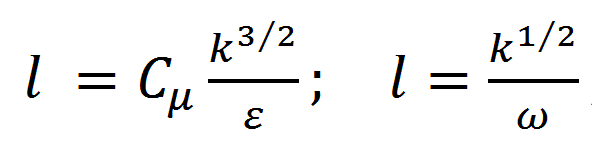
Formulas for calculating the input pulsation parameters and turbulence scale
At the boundary conditions in turbulent flow, the determining parameters are set: TurbEnergy and TurbDissipation. TurbEnergy can be defined as Pulsations: TurbEnergy = Pulsations. A TurbDissipation as a turbulent scale: TurbDissipation = Turbulent scale
RECOMMENDATIONS FOR THE wall FUNCTIONS APPLICATION IN FV
Recommendations for the use of wall functions in FV are determined by the Y+ value. On the base of it we can formulate some recommendations on the use of turbulence models and the wall functions. However, it must be borne in mind that the limits of models applicability for different tasks may vary.
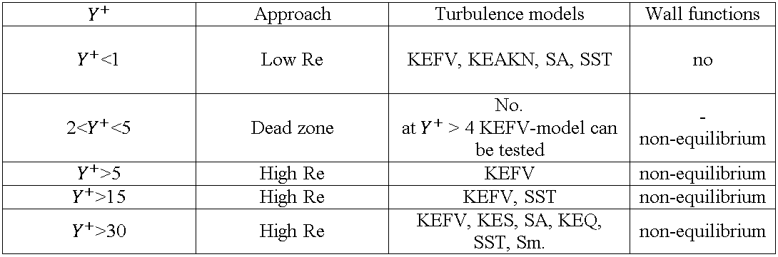
The equilibrium wall functions WFFV are set in the FV interface by default.