Characteristics are one of the most powerful tools in the FlowVision software complex for obtaining information about the calculation.
Characteristics can be used to:
- obtain calculation results, such as: flow rate, pressure, temperature, or forces acting on a surface or in a volume section
- monitor calculation results, outputting the data as a graph within the program interface
- debug the project / diagnose problems (for example, by finding extreme values within the computational space).
What Are Characteristics
Characteristics are a set of integral values calculated on a selected Object. This can be:
- a standard FlowVision object: plane or box / sphere / cone / cylinder / line / sensor
- an imported object
- a supergroup created on a computational domain boundary or on the surface of a boundary condition
- free space within the volume.
Using Characteristics, you can obtain the value of a variable over a surface or volume of an object, as well as at any point within the domain.
How to Use Characteristics
You can view the output of created characteristics:
- in the info window at the current time step 
- in the monitor window as a graph over time
Characteristic values can be saved to a .glo file for further processing in third-party programs such as Excel, Origin, ParaView.
Characteristics can be calculated:
- within the volume of an object
- over the entire surface of an object
- on individual object surfaces (for example, on the base, side surface, channel surface, or cross-sections)
- along a line (In this case, characteristics are calculated for all cells through which the line passes)
- at a point (In this case, the characteristic tracks the variable values in the cell which contains the point)
Characteristics are useful when calculating secondary variables using the Formula Editor. This approach can be used, for example, to convert values from one numerical system to another.
Types of Characteristics
Internal Characteristics
By default, each project is created with “Internal Characteristics”, which contain information about the main parameters of the calculation: current time, iteration number, time step size, explicit time step value, reference temperature and pressure, gravity vector components. The data from these Characteristics is often necessary to define time or step dependencies in user-defined variables.
User Specified Characteristics
Custom characteristics can be created in both the Preprocessor and the Postprocessor.
Due to the sequencing of the FlowVision modular structure, characteristics created in the Postprocessor are not available for use in the Preprocessor
Let’s look at the features of characteristics created on various objects, and consider cases when they can be useful.
Characteristics Applied to Body Volume
These characteristics can be created on the Computational space or on volumetric objects (both stationary and moving).
Characteristics of this type make it possible to determine:
- extreme values of a variable within the volume
- coordinates of the cells in which these extreme values appear
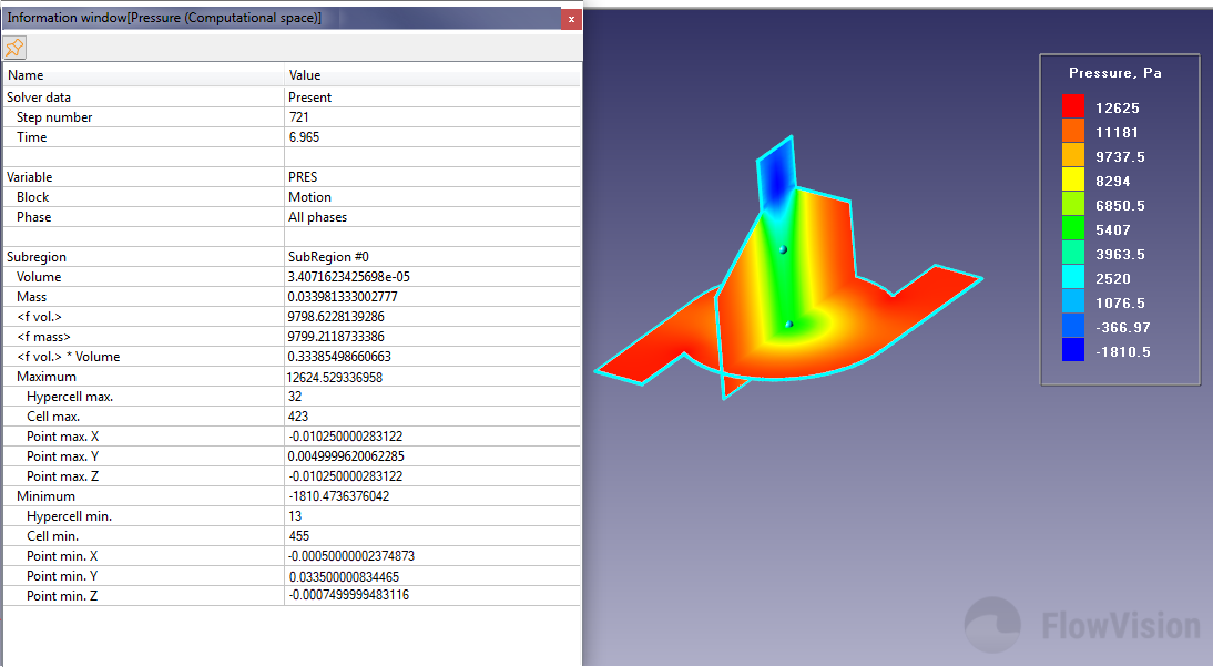
Info window for volumetric characteristics
In situations, when a solution "falls apart", it is necessary to analyse the solution to find problem areas within the calculation domain. It is possible to determine when and where the “collapse” of the solution occurs due to the fact that variables (pressure, temperature, density, Mach number, etc.) in some cells take on abnormally large/small values. When viewing the colour contours for these variables, the "bad" cells may not always be detectable with the naked eye. It is at times like these that Characteristics come to the rescue! Using Characteristics, it becomes possible to locate these cells and analyse what caused such values to be generated.
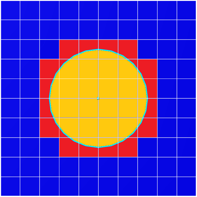
The volume of a characteristic applied to an object always differs from the true geometric volume of the object
When creating Characteristics, it is important to note that all cells that are intersected by the surface (or the object) are included in the characteristic’s calculation volume. Therefore, the calculation volume of Characteristics always slightly exceeds the volume of the object on which it is created.
Characteristics on a Moving Body
When creating Characteristics on the Imported object from which a Moving body is built, additional fields appear in the information window for the center of rotation, translational velocity, rotation speed, and the rotation matrix of the Moving body. If the body is in motion, these values are calculated and displayed. Otherwise, these strings are assigned a null value.
If you create a Characteristic on a Supergroup constructed from the surface of a moving body, then the fields related to the moving body that contain the calculated parameters of motion will be absent
Difference Between Characteristics Created on a Plane / Supergroup
There is a big difference between Characteristics created on a Supergroup on a boundary condition, and those created on a plane or object surface, exactly replicating that Supergroup.
The variable values for Characteristics created on a Supergroup are recorded from the boundary condition. But for Characteristics built on a plane / object surface, values are recorded from the centers of the control cells at the boundary. These values are almost always different.
Characteristic on a Selected Contour
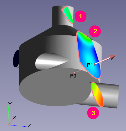
Let us consider a case when the plane on which a Characteristic is constructed passes through several calculation subregions or forms several closed contours. Then the question arises, what exactly does the characteristic calculate on such a plane?
If the plane intersects several calculated subareas, then when calculating the Characteristics on the plane, the subregion is selected in accordance with the position of the reference point.
If the plane intersects the geometry of the subregion in such a way that several closed contours are formed, then:
- by default, the characteristic is calculated across all contours
- you can select a single contour across which the characteristic will be calculated
To do this, place the reference point inside the contour of interest and select ‘integration along the selected contour’ in the Characteristic properties.
Other features of plotting Characteristics on a plane are described in the documentation.
Characteristics on a Set of Sensors
In FlowVision, you can get variable values at specific points within the computational space. To do this, you need to create the standard object “set of sensors”, and then create a characteristic on it. The value of the variable in the cell containing the sensor is transferred to the Characteristic. The information window of characteristics created in this way will contain values from all sensors.
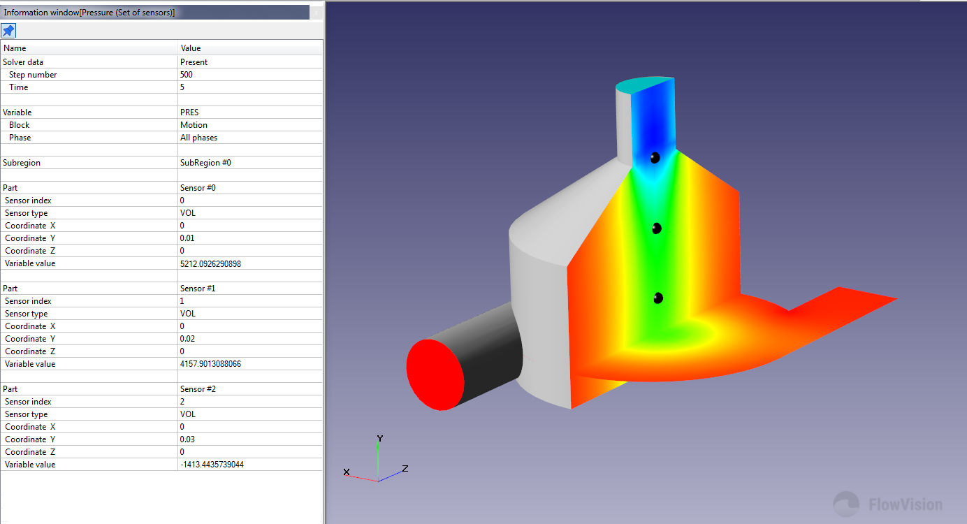
Info window for Characteristics based on a Sensor Set
Exporting Characteristic Results
If data obtained through Characteristics needs to be exported to third-party programs (to plot as graphs in Excel, for example), then this can be done by specifying the appropriate save settings in the properties window for the required Characteristics in the Postprocessor tab.
Characteristics are saved to text files with the .glo extension, which are stored and overwritten in the server part of the project. A detailed description of the output file can be found here.
We recommend that you always save the calculation results of the characteristics defining the task.
If you need to look at the calculation history of the calculation and at the parameters of the Characteristics at the current and previous time steps, then it will suffice to simply open the file in Excel and look at the values.
If data autosaving is enabled, then it is possible to create a new characteristic and calculate its values over the previous steps. This can be useful if you want to get the dynamics of some value when the calculation has already been completed. To do this, you need to create a new characteristic at the last iteration, configure its saving to a file, and load the results for the first (or any previous) iteration. If you want to calculate the Characteristic value over only one iteration, on the toolbar, click  . If you need to calculate the Characteristic value for all saved previous iterations, then click
  and reload all steps.
If the .glo file is open while the project calculation is running, then the Characteristics data will not be written to the file.
Due to the specifics of the file system, on Linux versions, Characteristics may not be saved if their name contains cyrillic characters.
A Demonstration of Using Characteristics on the Mixer Example from the Tutorial
Let's consider the main capabilities on a simple typical FlowVision example - namely, the mixer. The complete project is detailed in the Quick Start section of the FlowVision documentation.
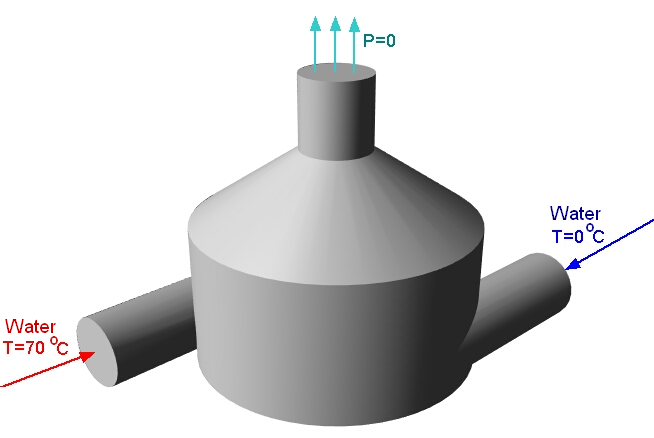
In this task, there are two inlets: one for cold water, the other for hot, and the outlet is located at the top of the mixer. For the two inlets, we assign the boundary condition (BC) - normal mass velocity; and for the mixer outlet - zero total pressure. In order to be confident that the solution has converged and reached a stationary state, it is necessary to track the dynamics of changes in variables over time. If they do not change over time, then the calculation can be stopped. In the given task, it is reasonable to monitor the average velocity and temperature at the mixer outlet. It would also be useful to track the flow rate balance to make sure that our Phase does not “leak” anywhere, and that the amount of fluid introduced into the calculation domain is equal to the amount of fluid leaving it. We will accomplish all this using Characteristics.
We will not be applying a turbulence model. The selected grid is 20x20x20, the time step is 0.01 seconds.
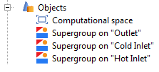
To begin, you need to create three Supergroups: a Supergroup for “Hot Inlet”; a Supergroup for “Cold Inlet”; and a Supergroup for “Outlet”. We do this according to the corresponding Boundary Conditions.
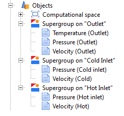
Then, for each Supergroup, we create characteristics for the variables which are of interest. For both of the Inlets let's create two characteristics - pressure, and speed. For the Supergroup on “Outlet”, create characteristics for pressure, speed, and temperature.
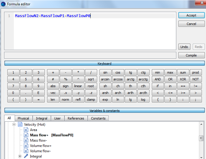
Another application of Characteristics is to calculate secondary variables using formulas set by user variables. Let's look at an example of how to do this. Let’s say we want a Characteristic, which will contain the result of calculating the difference between the flow rate at the outlet of the mixer and the flow rates at the hot and cold inlet. To do this, first create a custom variable in the PrePostProcessor tab. Let's call this variable “Flow rate difference” and use a formula to set its value.
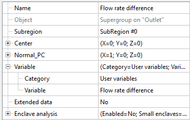
Then it is necessary to create a Characteristic on the Supergroup object for “Outlet”. In its properties window in the Variable>Category field, select “User variables”, and in the Variable> Variable field, select our created variable “Flow rate difference”.
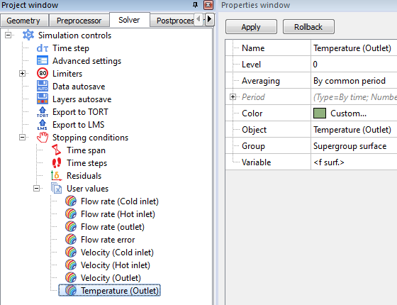
Next, go to the Solver tab> Stop Conditions> User Values and create seven stop criteria. In the properties window of each Stop Criterion, set the corresponding object - the Characteristic based on which the calculations will be made.
To calculate the velocities at the selected BCs, select <f surf.> in the “variable” field. This will calculate the average value of the variable over the whole surface. Similarly, calculate the average outlet temperature. View the documentation for a more detailed description of additional features of FlowVision, as well as of the purpose of the other items in the variable field (such as <f mass +>, <f mass->, Standard deviation, Heat flux [W], etc).
We end up with the following stop criteria:
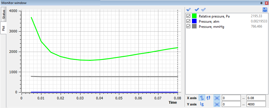
This completes the preparation of the calculation. After starting the calculation, all of these values can be monitored in the Monitor Window.
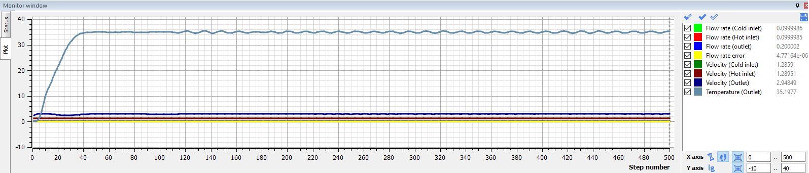
You can select a variable of interest and monitor only its value alone. For example, consider the graph of the change of the average outlet temperature with time.
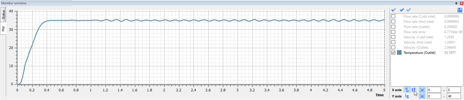
Looking at this result, it can be seen that the problem has already reached a quasi-static solution at 1.2 seconds, and that the average outlet temperature is about 35 degrees.
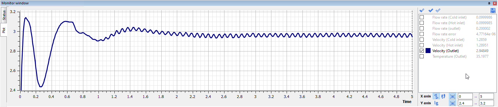
However, the outlet velocity stabilized only at 2.4 seconds, and is approximately equal to 2.9 m / s:
The mass flow balance was slightly off zero initially, but at 0.6 seconds it has already leveled off and is fluctuating around zero:
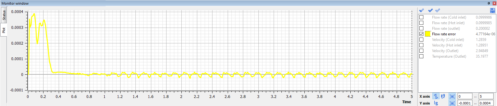
The resulting graphs are unsteady. This is due to the fact that when preparing the model for calculation, it was chosen to use a large time step and a coarse mesh.
In this task, in order to achieve complete convergence, it is necessary to refine the mesh and decrease the time step. Then the values of the Characteristics will eventually assume constant values.
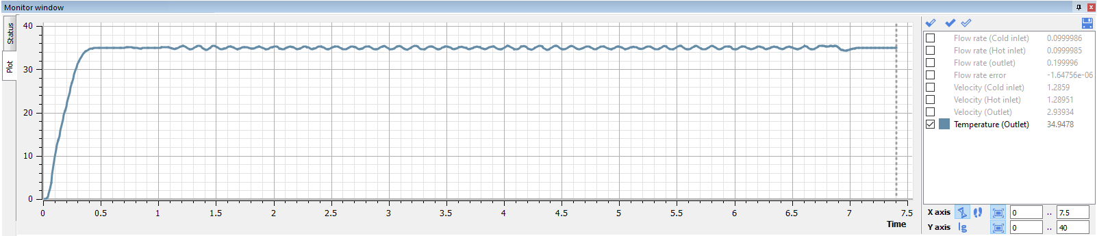
Notice the resulting change in the average temperature over the outlet section after changes were applied (at 6.5 seconds the mesh was refined and the time step reduced).
The solution has completely stabilized, and at 7 seconds the average temperature has already settled on a constant value.