Today we will talk about minimization of the computational mesh in a two-dimensional calculation. In general, FlowVision is a three-dimensional CFD software. But the 3D calculation becomes 2D if there is only one calculation cell in one direction. Unfortunately, two-dimensionality disappears when adaptation is enabled. User of FlowVision from JIHT figured out this issue.
mesh refinement and adaptations
There are two ways to refine the mesh near the profile of a streamlined object in FlowVision:
- Using the refinement of initial mesh (non-uniform initial grid)
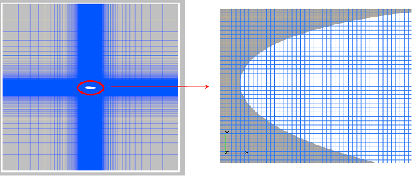
The size of the cubic cell face near the profile is 0.0025 m.;
Initial mesh contains 198 x 178 x 1 cells;
The number of cells of the computational mesh is 34 628.
- Using adaptation (for example, surface adaptation)
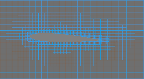
The size of the cubic cell face of 3 adaptation levels is 0.0025 m;
The initial mesh contains 64 x 60 x 1 cells;
The number of cells in the computational mesh is 16 580.
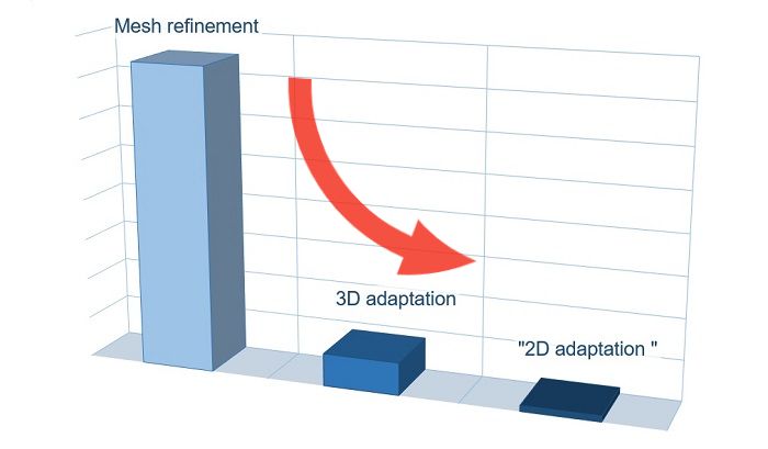
The adaptation allows reducing the number of computational cells by 2 times while maintaining the same cell size of the profile surface!
But we have moved away from the 2D statement of the task. After applying the adaptation not only one cell is located in the thickness of the computational domain.
flowvision adaptation is always three-dimensional
Adaptation is a three-dimensional division of a cell into 8 identical parts.
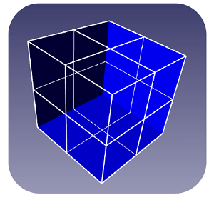
What happens when you turn on the adaptation of level n in the project? The cell located by the thickness of the computational domain is divided into 2n parts. Therefore, the size of the computation grid grows somewhat faster than we would like to have for two-dimensional calculations.
But there is a way to solution. It will be possible to transform three-dimensional adaptation to two-dimensional by modifying the project. Now there always is only one cell in the thickness of the computational domain despite the adaptation.
Using a non-computational subdomain at a distance from the computational one
Let's describe solution algorithm step-by-step using the the FlowVision tutorial task "Flow around the NACA profile".
To start with, open the project and run the calculation. The number of calculation cells is equal to 588 496 in the monitoring window. Note: the number of the initial grid cells in the Z direction is set equal to 1 in interface. When calculation is running, we can see that it increases to 8. This happns because adaptation is enabled and cells are adaptating in all directions.
Now we will demonstrate how to reduce the number of cells in a two-dimensional statement.
step 1
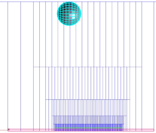
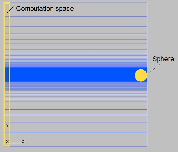
Create an object (for example, a sphere) and place it at a distance from the calculation plane. This distance is calculated by the formula: 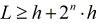 , where n is the maximum adaptation level setted in the project.
 step 2
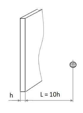
In the context menu of the created sphere, select "Build in the main geometry".
As a result, a new Subdomain will appear. We don't set a Model in it. Then the subdomain will remain non-computational and the initial grid will just be longer in the perpendicular direction to the calculation plane direction.
step 3
Check up in the properties window of the initial grid that only one cell is setted in z-direction. All cells in this direction are very elongated, but this will not affect the accuracy of the calculation. The real calculation cell is one that is cut off from the initial cell by two symmetry planes. Thus, the initial grid in the computational area is close to the cubic one.
step 4
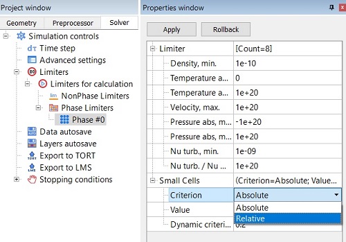
Change the criterion of cells smallness from absolute to relative. Otherwise, the entire volume will be filled with small cells due to the fact that actual cells are significantly smaller than the initial ones .
If this would not be done, all small cells will merge into one large calculation cell and the computational area will not be resolved by grid.
step 5
Check up if the adaptation is active and the calculation started . The grid adapts in all three directions as it has ben before, but in Z direction the cells are split outside the computational area. As a result, there is always only one cell in the thickness. Therefore, the total number of calculation cells is 2 times less than in our first calculation, namely 288 798 cells.
Сross section according to the thickness of the mesh is shown below. The red rectangle is the cross section of the calculated area, and the green line is the edge of the last adapted cell (the maximum adaptation level). The figure shows that the thickness of the computational domain consists from only one cell despite the adaptation.